Post process - UQ

The UQ method automatically converges to a correct solution, i.e. accurate final Probability Density Function (PDF). However, one can be interested in the convergence of the process, which is divided into two aspects. The first aspect represents the selection process of important increment functions, which is done with our prediction scheme. The second aspect represents our adaptive scheme, which optimally samples each increment function. Our adaptive scheme differentiates between the convergence of the final model (global convergence) and the convergence of each increment function.

Theory behind#

Prediction scheme#

The first step in the approximation process represents the selection of important increment functions, i.e. domains that play a crucial role in the process of approximation. Selecting only important increment functions leads to accurate and cheap approximation. Once the prediction scheme is converged, a linear model is selected to approximate the remaining residual. In other words, we are considering only increment functions which are neglected (not used) in the final model. This linear model is called the Linear model of residuals.

Our prediction scheme deselects increment functions based on their statistical influence and only the important increment functions are selected, i.e. increment functions having influence higher than the residual defined by the user. This allows for reducing the number of required samples and such that speeds up the interpolation process.

Our code is designed to consider only increment functions, which could be useful in the process. However, it can happen that the sum of the increment functions with extremely low influence can in total lead to a significant change in the final PDF. For example, the user-set residual is $0.05$ and increment functions $dF_{1.2.3}$ , $dF_{1.2.4}$ , $dF_{1.3.4}$ , $dF_{1.2.3.4}$ have influence around $0.0001$ each. This is significantly lower than a user-defined residual and adding these increment functions would cost an additional 54 samples, which is a very high price. Therefore, these increment functions are neglected. The influence of these increment functions is caught with our linear residual model. Therefore, we let the user decide if these increment functions are needed. If one wants to include these increment functions simply reduce the global residual and re-run the learning process. It should be kept in mind, that this will lead to a larger number of samples required.

The linear model is selected due to the assumption that the least complex model capable of performing statistical propagation is linear. In other words, any complex function can be approximated with a linear model, if its influence is negligible. In this case, the linear model serves as an estimator of residual. Therefore, adding the results of the linear model to the final model serves as an estimator of the influence of the neglected increment functions. One can consider the function as converged if a change in the final distribution is negligible.

NOTE

For non-normal distributions, large values of variance for the linear model can lead to a very small change in the final model. Therefore, it is suggested to visually check the final distribution.

A very important aspect of the linear model is its conservatives. In other words, in reality, the real influence of neglected increment functions will be lower than predicted by the linear model. Thus, one can expect only smaller changes in the final model than predicted by the linear model. Another property of the linear model is that it naturally converges to zero if all increment functions are used. Therefore, the residual of the model diminishes as more increment functions are included in the final model.

Adaptive sampling convergence process#

Global convergence#

This type of convergence is commonly known and understood. In each iteration, once the samples are added to the domain and the final model is built, the final model is checked if it is accurate enough, i.e. the residual of the expected value and the variance is below the given threshold. The equation for the residual of the expected value reads:

R_{\mu}=\frac{\left|{_p}\mu-{_{p-1}}\mu\right|}{\left|{_p}\mu\right|}

and the residual of the variance reads:

R_{\sigma^2}=\frac{\left|{_p}\sigma^2-{_{p-1}}\sigma^2 \right|}{\left|{_p}\sigma^2 \right|}

where $\mu$ represents the expected value, $\sigma^2$ represents the variance and the subscript (in front of the letter) $p$ represents the iteration. The model is considered converged once both residuals ( $R_{\mu}$ and $R_{\sigma^2}$ ) are below the given threshold, i.e. fulfil the prescribed criteria.

NOTE

To maximize the gain of each sample, most of the samples are used in the final model. The infamous over-fitting phenomenon is handled inside the developed code and the handling scheme is part of the internal know-how of the Uptimai company.

Convergence of increment function#

This type of convergence represents the convergence of each individual increment function - $dF$ . It consists of 2 convergence approaches - the normal convergence and the logic convergence. The normal convergence for the expected value of a given increment function is defined as follows:

R_{\mu}=\frac{\left|{_p}\mu_k-{_{p-1}}\mu_k \right|}{\left|{_p}\mu \right|}

and the normal convergence for the variance of the given increment function reads:

R_{\sigma^2}=\frac{\left|{_p}\sigma_k^2-{_{p-1}}\sigma_k^2 \right|}{\left|{_p}\sigma^2 \right|}

The logic convergence for the increment function is defined in the following way:

RL_{\mu}=\frac{\left|{_p}\mu_k-{_{p-1}}\mu_k \right|}{\left|{_p}\mu_k \right|}

and the normal convergence of the variance for the given increment function reads:

RL_{\sigma^2}=\frac{\left|{_p}\sigma_k^2-{_{p-1}}\sigma_k^2 \right|}{\left|{_p}\sigma_k^2 \right|}

where $\mu_k$ represents the expected value of the $k$ increment function, $\sigma_k^2$ represents the variance of the $k$ increment function and the subscript (in front of the letter) $p$ represents the iteration. Notice the difference in the denominator for the normal and logic convergence. The increment function is considered converged if either logic or normal convergence criterion is reached. However, both residuals, i.e. for the expected value and variance, have to be below the given threshold to consider the increment function converged.

The difference between normal and logic convergence is that the normal convergence process takes into account the behaviour of the model, while the logic convergence only observes the given increment function. This helps to optimize the number of samples used for the model creation, and it makes the process robust. For example, consider a problem, where the final model is diverging. In that case, adding samples to the converging increment functions is pointless. In this problem, the logic convergence process ensures that samples are not added to an already converged problem (null improvement for the final model) and the algorithm focuses on the diverging increment functions. On the other hand, the normal convergence process ensures that samples are not added to the non-influential increment function. Consider a problem, which is converging and the given increment function has a very low influence. Adding samples to this increment function would lead to non-optimal samples with little influence on accuracy. Thus, the increment function does not need to be sampled further. The combination of these two convergence processes brings the optimal number of samples for the desired accuracy.

How to use the interface#

There is a collapsible box on the left side of the tab with the opened result file, where the user can set the data to be displayed. There is a list of clickable items showing the plot on the right. The type of the plot depends on the selected item. Prediction shows the histogram of the Linear model of residuals predicting the error estimation of the model. The Global item and items labelled with increment function designation show the linear plot describing the steps of the Adaptive sampling convergence process.

Linear model of residuals#

The plot presents the overlap of two histograms. There is the final probability density function of the modelled output (labelled as Original Model) and the final PDF enhanced by the linear model of residuals (labelled as Original + Residual Model). Their difference may suggest the model is missing some increment functions to achieve better precision.

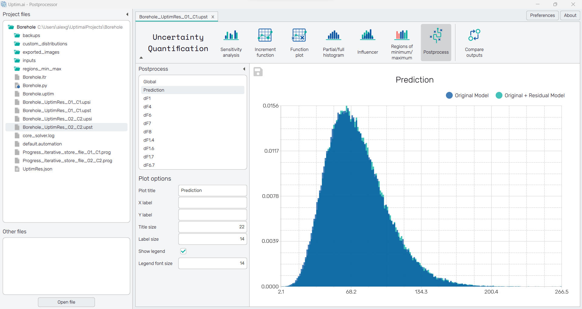
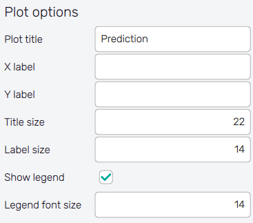
To save the histogram plot as a .png or .jpg file, the save-file dialogue can be induced by clicking the 💾 icon on the top left of the plot. It is possible to adjust the appearance of the plot using controls from the Plot options section of the panel on the left:

Plot title : Displayed above the plot, Prediction by default.
X label : Label of X axis, empty by default.
Y label : Label of Y axis, empty by default.
Title size : Size of the title font.
Label size : Size of the label font.
Show legend : Switching on/off the legend of the plot/the colorbar scale.
Legend font size : Size of the legend font.

Figure 2: Postprocess (Prediction model) - Plot Options

Adaptive sampling convergence process#

The linear plot shows the convergence process from iteration to iteration of the adaptive sampling. Users can recognize two sets of data: the convergence of the Mean value and the convergence of the Variance of the final probability density function of the model. One can use three buttons under the list of increments to display either the Convergence of absolute mean and variance values, the Residual total stating the absolute value of residual, or the Residual logic for its normalized value (not available for Global residuals).

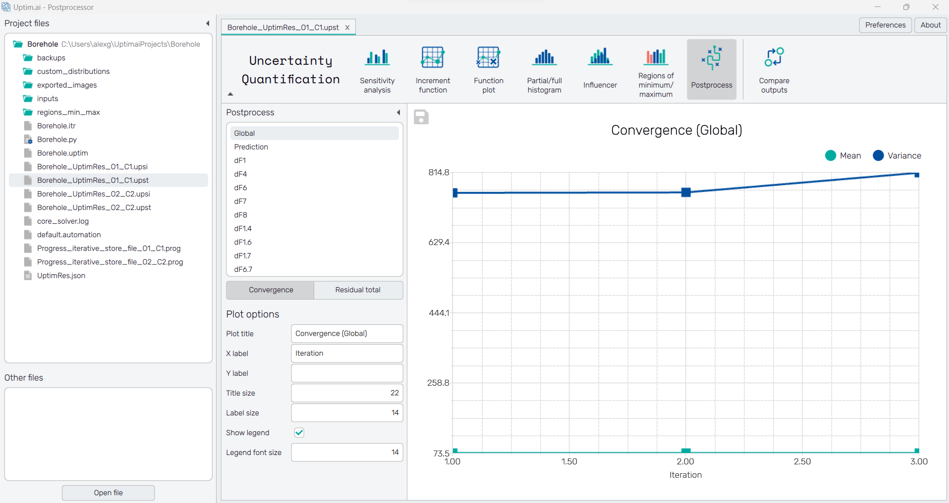
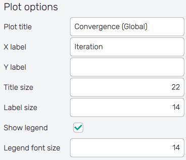
To save the convergence plot as a .png or .jpg file, the save-file dialogue can be induced by clicking the 💾 icon on the top left of the plot. It is possible to adjust the appearance of the plot using controls from the Plot options section of the panel on the left:

Plot title : Displayed above the plot, Convergence (global) or increment function designation by default.
X label : Label of the X axis, Iteration by default.
Y label : Label of the Y axis, empty by default.
Title size : Size of the title font.
Label size : Size of the label font.
Show legend : Switching on/off the legend of the plot/the colorbar scale.
Legend font size : Size of the legend font.

Figure 4: Post process (convergence) - Options