Home screen

Uncertainty quantification is the science of quantitative characterization and reduction of uncertainties in both computational and real-world applications. It tries to determine how likely certain outcomes are if some aspects of the system are not exactly known. Every system is influenced by uncertainties and using a proactive approach, the most influential uncertainties can be overcome with slight modifications of the initial design.

Theory behind

Our program is a non-intrusive uncertainty propagation approach and it is based on the High Dimensional Model Representation (HDMR), where each sub-function is treated independently. Each sub-function is called \"increment function\" and as its name suggests, it adds a small increment to the nominal value. The nominal sample (or nominal value) can be understood as an initial design around which are uncertainties observed. In the mathematical formulation, the HDMR reads:

$$F(x_1,...,x_n)=F(^cx_1,...,^cx_n)+dF_{1}(x_1)+...+ \\dF_{1.2}(x_1,x_2)+...+dF_{1.2.3}(x_1,x_2,x_3)+...+dF_{1...n}(x_1,...,x_n)$$

where $F(\bf{x})$ represents the function of interest, superscript (in front of the letter) $^c$ in front of variable $x_i$ represents the nominal position of variable $x_i$ and $dF$ represents the increment function, which is defined in the following way:

$$dF_{1...n}(x_1,...,x_n)=\int_{^cx_1}^{x_1}... \int_{^cx_n}^{x_n} \frac{\partial F(\mathbf{x})}{\partial x_1 ... \partial x_n} dx_1...dx_n$$

However, working with integrals and derivatives is not convenient and therefore, the increment function is transformed into the analytic form, which reads for the first order:

$$dFi(x_i)= F(x_i,^c\mathbf{x})-F(^cx_i,^c\mathbf{x})$$

for the second order, it reads:

$$dFi.j(x_i,x_j)= F(x_i,x_j,^c\mathbf{x})-F(^cx_i,^c\mathbf{x})-dFi(x_i)-dFj(x_j)$$

and the higher-order increment functions are defined accordingly.

The order of the increment function is given by the number of functional variables as it is shown above. The function of interest is fully defined with all increment functions, however, this represents an extreme computational burden, e.g. for a 3-D problem, it would be 125 samples of the expensive solver using only 5 samples per abscissa. Therefore, only important increment functions are selected using our selection scheme and such reduces dramatically the number of samples. The neglected increment functions are considered to be zero, i.e. they have a null influence on the final uncertainty. The selection scheme is part of the internal know-how of the Uptimai company.

Each increment function is interpolated/approximated with an independent model and the sum of these models creates the final interpolation/approximation model. Currently implemented surrogate models are:

• Lagrange interpolation : Well-known technique for simple functions.
• ISI : ISI stands for Independent Surrogate Interpolation and it is used for complex functions involving highly oscillatory and discontinuous regions. ISI interpolation technique is part of the internal know-how of the Uptimai company.
• ANN : ANN stands for Artificial Neural Network. It was incorporated to deal with the simulation of interconnected processes and extremely complex problems.

The selection process for each model is fully automatic, i.e. the algorithm selects the best model for a given problem. This ensures that the process is efficient but also very robust, thus, the final model does not diverge. The selection process is part of the internal know-how of the Uptimai company.

This final surrogate model is used to propagate Monte Carlo (MC) samples establishing the final statistics for the selected problem. However, partial statistics can be obtained by the application of MC directly to the interpolation model of the increment function. This allows to establish the statistical influence of each increment function and to gain further insight into the problem. The application and use of each increment function are described in each section under Uncertainty Quantification.

A very important aspect plays the nominal solution, $F(^cx_1,...,^cx_n)$, which represents the deterministic solution for given nominal values of input distributions. The nominal sample (or solution) is defined in the preprocessing phase and by default, it is positioned in the mean value of a defined distribution. The nominal solution can be understood as a result, which would be obtained if the statistical approach had not been taken.

NOTE

The nominal solution can be selected arbitrarily. However, to have an easier explanation of the results, it is suggested to use the mean value of the input distributions as a nominal sample.

How to use the interface

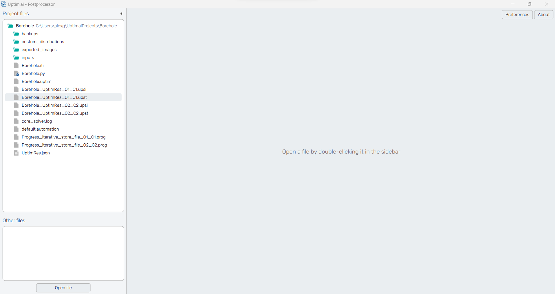
In Figure 1, it can be seen the initial state of the application's window, which is split into two sections. On the left side of the window there is the Project files frame showing the file structure of the current project folder. The frame itself is collapsible by the mouse clicking on its label or the < symbol. The user can open and close subfolders shown in the directory tree by double-clicking.

Figure 1: Result Postprocessor - Main window

Double-clicking also opens files to be shown in the Postprocessor, here is the list of currently available supported file types. Opened file appears in the right section of the window as a new tab. Another way to open a file is through the right-click menu, accessing the following features:

• Open : Opens the file in the same way as in the case of double-clicking it in the project directory tree.
• Open in New Tab : Always opens the file in a new tab. Unlike the standard Open method, this one allows to show multiple tabs with the same file. This is helpful when multiple postprocessing features of the same file need to be seen next to each other.
• Open in Right Split : Directly splits the workspace and arranges the new tab to the right from an existing one.
• Open in Default App : Opens the file in the system default application for the type. Useful for file types not featured in supported file types, especially for non-Uptimai files.
• Compare Outputs : Starts the dialogue of the dedicated feature where the user can directly compare the results of two outputs of the project and their statistical properties.

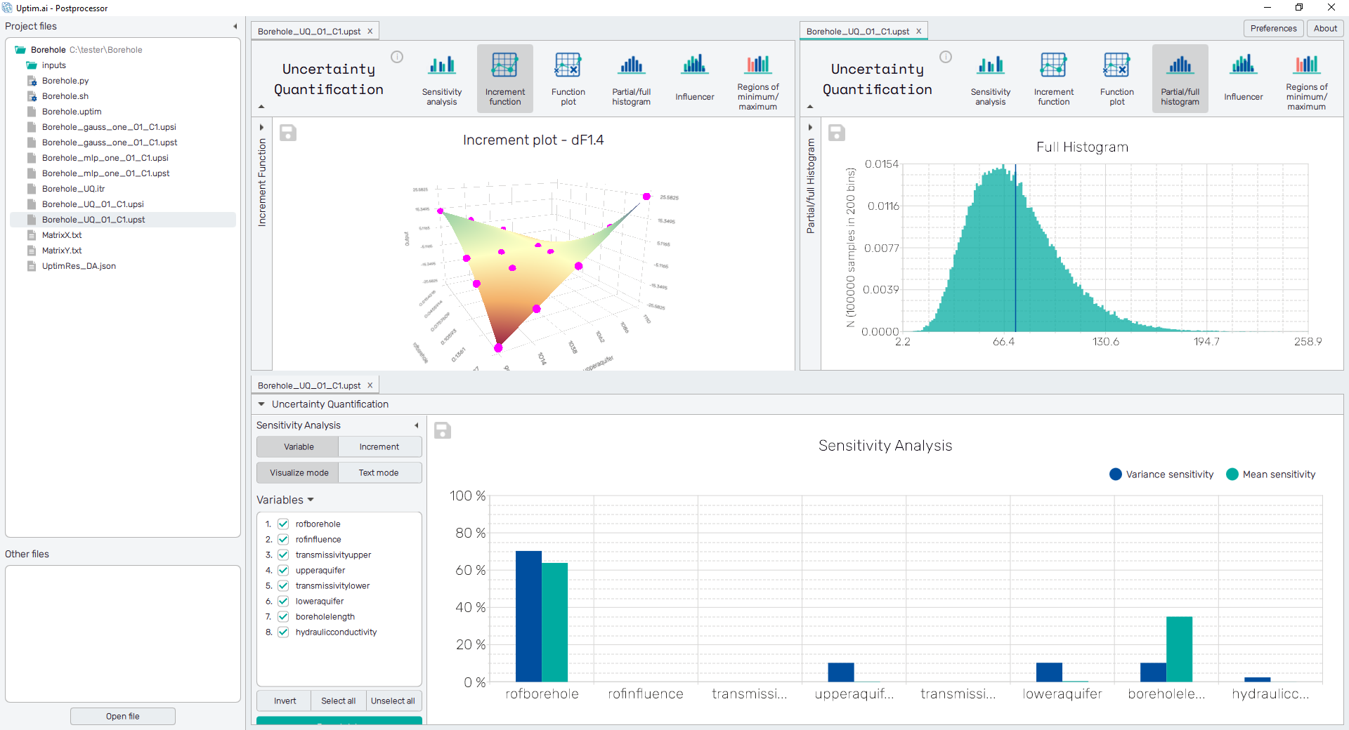
The general appearance of the tab is shown in Figure 2. Each tab has its label on the top together with the X symbol closing the tab. When multiple tabs are open, they can be rearranged with mouse-dragging of their labels to observe more than one file at a time. If one of the Uptimai result files is opened, a bar with postprocessing features is shown on the top of the tap. The bar also shows on the left if the opened file was identified as an Iterative file or refers to the
method used to build the model in the result file.

Figure 2: Result Postprocessor - Arrangement of tabs

The right top of the screen holds two additional buttons. The Preferences button opens the dialogue with the setting of the general behaviour of the Postprocessor. Users can enable the Multiprocessing to speed up features of the program, mainly the process of model interpolations. The About button shows the menu dedicated to accessing the link to this document (Help), contacting Uptimai company to get the support (Company), and showing the information about the currently installed version of the program (Version).

List of Postprocessor features

The Postprocessor offers a variety of features for data analysis and plotting. These are accessed through icons shown in the bar at the top of the tab with the opened file. The list of features currently available for the opened file may vary based on the method used by the Uptimai Core Solver, and according to the filetype which is currently opened. All features included in the program are:

• Sensitivity analysis : Sensitivity analysis tries to establish the influence of the input variable on the output of a mathematical model or system (numerical or otherwise). Based on the results of the sensitivity analysis, inputs relevant to the problem can be focused on.
• Increment function : Increment function plot visualizes the influence of a selected increment function. Each increment function represents a separate increment to the final model caused by uncertainties in the selected dimension (or combination of dimensions) of the domain.
• Function plot : Function plot is used to visualize the behaviour of the function of interest. Shows absolute output values through the design space, either as a value for a specified combination of inputs or as a function of up to three selected input variables.
• Partial/full histogram : A histogram is a representation of the distribution of numerical data. It is an estimate of the probability distribution for an uncertain output/s. This allows visualizing how each part of the variable influences the final distribution.
• Influencer : Influencer compares the final distribution against a distribution with selected increment functions or input variables neglected from the final model. This allows a comparative visualization of the influence of the aspects on the statistics of the problem.
• Regions of minimum/maximum : Regions of minimum and maximum represent a statistical approach to optimization. Distribution shapes of input variables proposed here follow general trends in the mathematical model and result in probability distribution shapes with either decreased or increased mean value.
• Postprocess : Postprocessor shows the convergence history of the mathematical model learning process. Also, it contains the data about precision approximations.
• Compare outputs : Direct comparison of two different outputs of the same project. This feature opens a new tab since another set of postprocessing features is available for comparison. The user needs to be sure that compared .upst files are based on the same set of inputs.
• Tabular view : Tabular view of the database of computed samples called in the process of the mathematical model learning. Allows to edit the database and export it into plain text format or .xlsx.
• Scatter plot : Scatter plot of function values of samples in the Iterative file database. Shows the basic correlation of outputs and their general relation to input variables.
• Optimized histograms : Optimized histograms are the result of the Statistical Optimization method, proposing new domain ranges to achieve prescribed optimization criteria. Users can see probability distributions of input variables used in each iteration of the optimization process and related distribution functions of interpolated function values.

Supported file types

The primary purpose of the Uptimai Postprocessor is to open and read files generated using the Uptimai Core Solver. These contain the surrogate mathematical model and the data necessary for its analysis. These are:

• .upst : Store file containing the mathematical model. It is generated at the end of the Uptimai Core Solver computation. It provides the data required for the evaluation and plotting of the results. These may vary according to the method of the solver.
• .upsg : Store file related to the Statistical Optimization method.
• .itr : Iterative store file containing the database of computed samples called in the process of learning the mathematical model. This database can be used to restore, check, and repair the model-learning run.

Besides, the Postprocessor can read some of the generally used types of files, such as pictures, plain text files and comma-separated tables, Python and shell scripts, and some others. A list of supported formats can be found below:

• .txt
• .csv
• .jpg/.jpeg
• .png
• .py
• .json
• .sh/.bat
• .stl