Variable

Sensitivity Analysis tries to establish the influence of the input variable on the output of a mathematical model or system (numerical or otherwise). This is a crucial aspect when the sensitivity of a system to uncertain geometry, material properties, manufacturing tolerances, etc. needs to be determined. Based on the results of the sensitivity analysis, inputs truly important for the design can be focused on.

Theory behind

The sensitivity analysis is performed with the Monte Carlo analysis applied directly to the final model and each increment function independently. The sensitivity of the variable takes into account all increment functions, which belong to the given variable. For example, variable $X_2$ considers increment functions that have the number '$2$' in their description, e.g. $df_2$, $df_{1.2}$, $df_{2.4.5}$ etc., and these increment functions influence the domain of variable $X_2$. This type of sensitivity analysis is similar to commonly used sensitivity analysis. However, there is a difference between variable and increment sensitivity. Increment sensitivity only includes the influence of a given sub-domain (increment function of a variable OR its interaction), while the variable sensitivity takes into account all the aspects of a given variable (increment function of the variable AND ALL its interaction effects).

In this program, we define two sensitivities for a variable. The first sensitivity is the sensitivity of the mean value, which represents the influence of a given variable on the final expected value. In other words, how the selected variable influences the statistical expected value of a given problem. The formula for the mean sensitivity reads:

$$SV_{\mu_{i}}=\frac{\sum_{k \in S_D}\left|\mu_k\right|}{\sum_{k \in S_T}\left|\mu_k\right|}$$

where $SV_{\mu_{i}}$ represents the sensitivity of mean for variable $i$, $S_D$ stands for the set of selected increment functions, i.e. all increment functions belonging to the variable $i$, $S_T$ represents the set of all increment functions and $\mu_k$ represents the expected value of $k$-th increment function.

The second type of sensitivity is the variance sensitivity, which represents the variable's impact on the final output. Variable variance sensitivity is defined as follows:

$$SV_{\sigma^2_{i}}=\frac{\sum_{k \in S_D}\left|\sigma^2_k\right|}{\sum_{k \in S_T}\left|\sigma^2_k\right|}$$

where $SV_{\sigma^2_{i}}$ represents the sensitivity of mean for variable $i$, $S_D$ stands for the set of selected increment functions, i.e. all increment functions belonging to the variable $i$ and $\sigma^2_k$ represents the variance of the $k$-th increment function. Computed sensitivities are presented in the program as Partial variance and Partial mean.

The variance sensitivity of a variable is not normalized and such that its sum does not give $1$. The reason is that some increment functions belong to multiple variables, e.g. $dF_{1.2}$ belongs to variables $X_1$ and $X_2$. The mean sensitivity is related to the standard deviation of the probability distribution of output values. This measure prevents input variables from being overrated due to improper scaling.

How to use the interface

There is a collapsible box on the left side of the tab with the opened result file, where the user can set the data to be displayed. Variable and Increment buttons on the top switch between two datasets described in the theory section. Below is the list of input variables of the project. When starting with variables, it is important to check increment functions later to find out if input variables are interacting significantly.

It is possible to include or exclude input variables from the set of displayed data via checkboxes next to each variable name. The selection of items can be also modified with three buttons under the list. The Invert button does the reverse action of all checkboxes in the list. Select all and Unselect all buttons turn all checkboxes on/off.

Two types of output are possible here. Either a tabular view induced with the Text mode button, or the barplot shown switched on by the Visualize mode button.

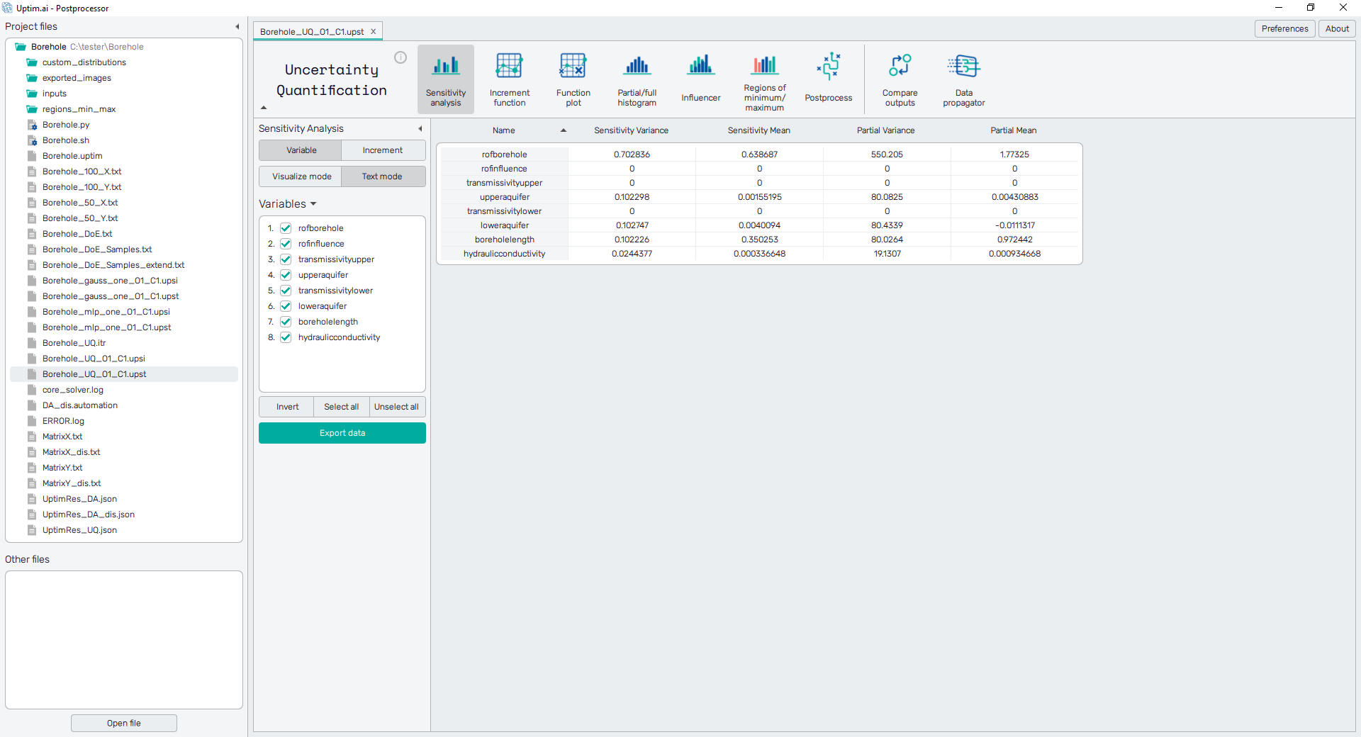
Text mode

The sensitivities of input variables are presented in the form of a spreadsheet, as shown in Figure 1. It is possible to change the sorting of the sheet(ascending or descending, where ascending is the default) by clicking on the row number or labels of sensitivities.

The green Export data button underneath the list of input variables saves the currently displayed data into a .csv or .txt file.

Figure 1: Sensitivity Analysis - Variable sensitivity in text mode

Visualize mode

In Visualize mode is the data presented in the form of a barplot, as shown in Figure 2. Users can see a graphical representation of sensitivities for each selected input variable. The sorting of variables in the plot is the same as in the selectable list of inputs on the left. The presence of mean sensitivities depends on the method used to create the .upst file - it is not available for the Preliminary Analysis method.

Figure 2: Sensitivity Analysis - Variable sensitivity in visualize mode

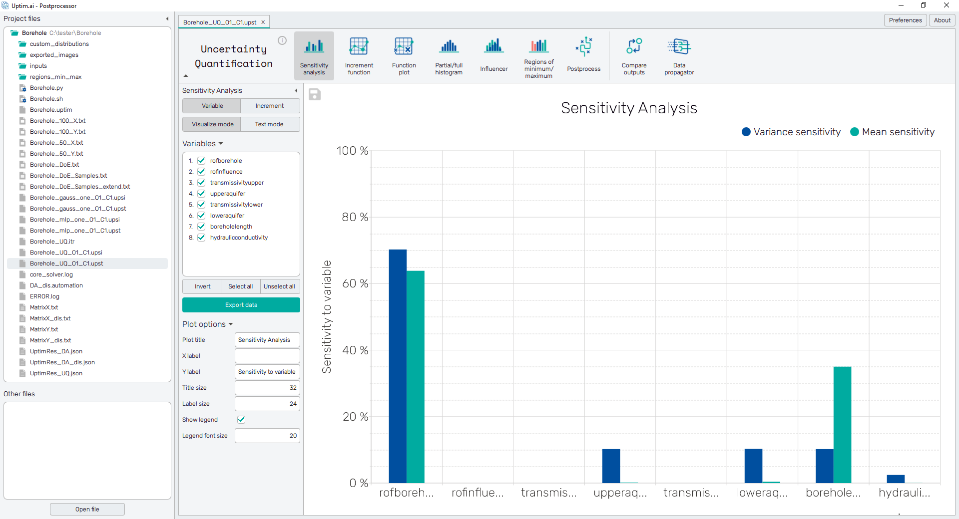
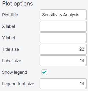
The green Export data button underneath the list of input variables saves the currently displayed data into a .png or .jpg file. The save-file dialogue can be also induced by the 💾 icon on the top left of the plot. It is possible to adjust the appearance of the plot using controls from the Plot options section of the panel on the left:

• Plot title : Displayed above the plot, Sensitivity Analysis by default.
• X label : Label of the X axis, empty by default.
• Y label : Label of the Y axis, empty by default.
• Title size : Size of the title font.
• Label size : Size of the label font.
• Show legend : Switching on/off the legend of the plot/the colorbar scale.
• Legend font size : Size of the legend font.

Figure 3: Sensitivity Analysis - Plot options of sensitivity analysis