Statistical Optimization

Uptimai Statistical Optimization gives the optimum zone of design of a given problem.

For doing that, it builds a set of models using the Uncertainty Quantification tool to capture and understand the effects and the importance of all variables and interactions in the different scales of the problem and with that knowledge reduces the initial domain of study up to a desired zone. This approach can find the optimum domain with a low number of samples, and more importantly, give a robust solution that performs well regardless of external uncertainties. The Statistical Optimization method will call for outputs corresponding to specific combinations of input parameters, thus, it is intended for work in connection with engineering computational codes etc.

How to use the interface

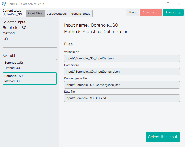
Figure 1 shows the initial screen of the Core Solver Setup GUI. The strip on the top of the window is common for all methods. From the left, at first, it informs the user about the setup file which is being processed. Then, there are three tabs of solver settings:

• Input Files : Here the user selects the set of inputs to be used and sees the list of corresponding files
• Cases/Outputs : The setup for the selected method and each solver run
• General Setup : The user can define the names of model result files as well as computational resources reserved for the Uptimai Solver

Figure 1: Core solver setup - Input Files tab for SO method

The control panel on top then continues with the About button with the menu dedicated to accessing the link to this document (Help), contacting Uptimai company to get the support (Company), and showing the information about the currently installed version of the program (Version). The Close button ends the preparation of the current setup (also includes the option to discard the data), and the Save setup button stores all changes to the *.json file. Also, there are ? icons on the solver setting tabs to show quick reference to the corresponding entry field or feature.

Input Files

The left section of the screen contains the general information about the Selected input. There is its name together with the Method to be used in the Uptimai Solver (in this case the Statistical Optimization) that was identified automatically from files of the selected input. Users can change the set of inputs (together with the method, eventually) from the list of Available items below.

When going through the list of available sets of inputs, the program shows their details in the right section of the GUI window. To choose a particular set of inputs as the currently selected one, double-clicking or confirmation with the Select this input button is required. When the reviewed input is the selected one, the aforementioned button is disabled and informs the user that This is the selected input.

Cases/Outputs

Here the user defines solver options for all cases in the current setup. Cases are listed in the left section of the program window, as seen in Figure 2. It is possible as many cases as needed, the Uptimai Solver will process them in the order prescribed by the list. The position of each case in the list can be changed by ist mouse-dragging by its = symbol. Clicking the X icon of the item will remove the case from the list. Other cases can be added to the list via the + Add case below the list.

Figure 2: Core solver setup - Settings of Cases/Outputs for SO method

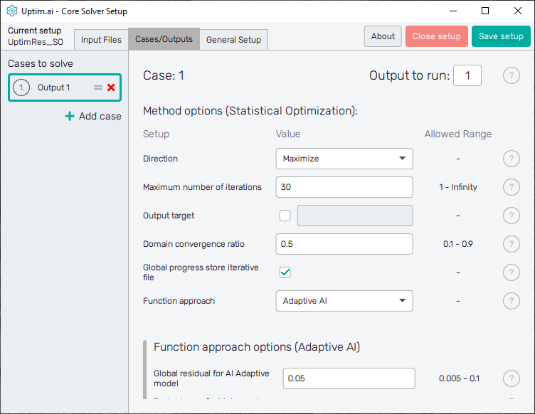
Cases in the list have generic names based on the project output which should be solved in the model. Clicking a list item highlights it in the list and the corresponding individual settings are shown in the right section of the window. The corresponding case number can be seen also on top of the right section of the GUI to ensure users with on which case they work. The top of the right section also contains the entry field where the Output to run is set. In other words, it is the column of the result matrix to be evaluated by the Uptimai solver.

Number of outputs

The Uptimai solver checks automatically the total number of outputs in the matrix of results by counting the number of columns. Be sure you are not calling the output number out of the existing range of columns in the matrix of results!

In the Method options below is the list of Setup entry fields, drop-down menus, or switches that are available for the Statistical Optimization method. Each entry field Value has to comply with the prescribed Allowed range. Options to be set are:

• Direction : The direction of the optimization shows if the optimization has to maximize (find the area with maximum output values) or minimize (find the area with minimum output values).

• Maximum number of iterations : The maximum number of iterations sets the limit value of iterations that the statistical optimizer has for reducing the domain between each model. The recommended value for general problems is 500. Nevertheless, for problems with very large numbers of samples, this value can be increased to ensure a better reduction of the space to the desired parameters.

  Note that this value does not have anything to do with the number of real samples that will be computed.

• Output target : The output target sets a threshold value that limits the desired output probabilistic distribution. In the case of maximization, the optimization process will continue until the minimum value of the shortened domain is higher than the selected output target. In the case of minimization, the optimization process will continue until the maximum value of the shortened domain is lower than the selected output target.

  If the output target is not selected, the convergence criteria regarding output limits won’t be used. For all cases, other convergence criteria are also used (maximum reduction of the space, total optimum found, etc.) in which case the limit may not be achieved.

• Domain convergence ratio : The domain convergence ratio sets the rate at which the domain can be reduced between every model. The recommended value is 0.5 (which means that the variables range can’t be reduced more than 50% per model). For simple problems it is recommended to use lower values, and for more complex models higher. Note that this value is directly linked to the number of models built and to the number of samples required for the optimization process.

• Function approach : It sets which model is used as the data source for the optimization process. It can be a model based on Data Analysis method, or an adaptively created model using the Uncertainty Quantification (UQ) approach.

  • Adaptive AI : Using an AI-driven adaptive modelling technique, the model is iteratively updated to converge toward the optimal design range.
  • Data model : Using the already existing model created with the Data Analysis method.

• Global residual for AI Adaptive : This number represents the relative residual, that is set for the mean value of the variance of results. The algorithm iterates until the residual is achieved for both observed values, i.e.: the mean value and the variance.

• Prediction residual scheme : The selection of important increment functions is driven by the prediction residual scheme. Currently, there are two schemes implemented. The Percent scheme measures the percentual influence of the selected increment function against all increment functions. The Distance scheme takes individual input distributions into account and measures the statistical influence of the neglected increment functions, i.e. what is the statistical effect of neglected increment functions on the overall result.

  The Percent scheme is more suited for problems where users want an accurate model over the whole stochastic domain. However, for large-dimensional spaces (15+), the Percent scheme is very conservative and leads to a large number of required samples. The Distance scheme is coupled with the input distribution types. Thus, it is more suitable for real-world problems.

  It is suggested to use the Distance scheme by default.

• Sampling scheme for prediction algorithm : Positioning the number of test samples for the prediction scheme (the scheme that selects important increment functions) that affects robustness and efficiency. Currently, three schemes are implemented. The first scheme takes two positions on the boundaries of the stochastic domain, the second scheme takes only one position on the boundary of the stochastic domain and the third scheme takes three positions on the boundaries of the stochastic domain.

  The first scheme was found to be the most robust vs. efficient. It works well for all the problems including problems with limited randomness, e.g. simulations with explicit FEM codes, DSMC simulations, etc. The second scheme is used when the problem is simple, with null randomness (pure deterministic solution) and one wants to limit the number of expensive computation calls. The third scheme is very robust since it uses three positions to test the influence of each increment function. This scheme should be used if a large portion of randomness is expected in the external code or measurements.

  It is suggested to use the prediction scheme 1 by default.

• Maximum increment order : The maximum increment order sets the maximum allowed order of increment functions in the model, higher order increments will be disqualified from the computation. One can use this option to force the Uptimai Solver code to stop at a prescribed order and make the convergence process faster. E.g. users do not need to see interactions of inputs, thus, they set the maximum increment order to 1. However, the post-process convergence check is disabled if the maximum order is reached.

  It is suggested to let the code select the maximum order and therefore set the maximum increment order to 0.

• Progress iterative store file : Enables storing the current progress of the learning algorithm, which can be restored in case of an unexpected collapse of the code. Loading the progress from a file may significantly decrease the overall wall-clock time of the repeated learning process. The progress iterative store file needs to be fully compatible with the project and the current solver settings, otherwise, the computation run will be stopped!

OLD FILES

The file is stored under a generic name Progress_iterative_store_file_Ox_Cx.prog that only differentiates the number of the output and its position in the sequence of cases to be solved. The existing progress iterative file has to be deleted when the settings of the learning process are changed. Uptimai Solver will not proceed from the progress iterative file which is incompatible with the current setup!

• Preferred batch size : Desired number of samples to be called per batch. The Uptimai Solver will attempt to merge batches, if possible, to meet this requirement. It decreases the number of batches (iterations) needed to build a surrogate model, however, the total number of called samples will be higher because of the reduced adaptivity of the Uptimai Solver. This setting is suitable when working with highly parallelized external software.

  Setting the value to $0$ turns the feature off.

• Percentage of close samples : The percentage of an input variable range for selection of an existing sample. If the new input variable bounds are proposed close enough (according to the percentage setup) to an existing sample, this sample will be selected as the new boundary value to further reduce the number of samples called in the next iteration.

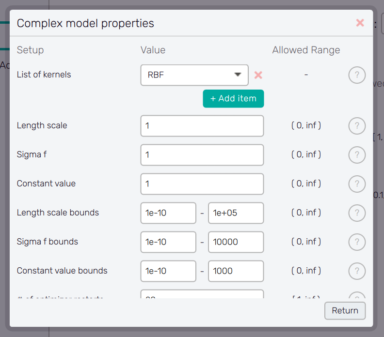
• Complex model type : A model that replaces a simple polynomial function when the underlying increment function becomes sufficiently complex. The solver automatically adapts to the problem, selecting the most accurate model.

  • Independent Surrogate Interpolation (ISI) : Well-suited for deterministic functions, as it passes through all given data points. It effectively handles highly complex functions but struggles with randomness or noise in the data.
  • Gaussian : The standard Gaussian process, with defined kernel functions and an added white noise kernel, preferable for handling noisy problems.

General Setup

The management of project results files and computer resources reserved for the Uptimai Solver is defined in the General setup tab.

Figure 3: Core solver setup - General setup of the Core Solver

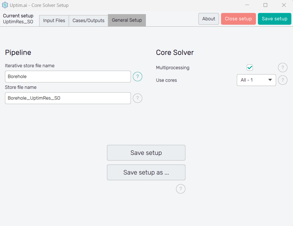
In the Pipeline section on the left can the user adjust the names of files where all results received from the solver run are stored. The Iterative store file name sets the prefix for the *.itr file that holds data values of all samples already collected from third-party software. The default basename is set as <project_name>. Store file name sets the naming convention for the final resulting file produced by the Uptimai Solver. This *.upst contains the set of statistical results of each individual model suitable for analysis in the Uptimai Postprocessor. The default basename is proposed as the <project_name> followed by the <setup-file_name>, the number of the output being solved, the number of the currently processed case and the iteration. For reference, see the default name of the result file of the project shown in Figure 3, where the second output was solved as the first case according to the solver setup:

Borehole_UptimRes_O1_C1_I00.upst

The name of the *.upsi file with the surrogate model suitable for processing through the separate Interpolant tool is composed in the same way.

In the case of the *.upsg file, where the information from all the models computed are shown together, the name convention is slightly different, adding Global_SO in the naming and not having the iteration number:

Borehole_UptimRes_Global_SO_O1_C1.upsg

The main goal of the proposed convention is to give a hint to the user on how to match the project files with particular settings of the Uptimai Solver just from the look into the file explorer.

The Core Solver section on the right of the window is about the number of CPU cores used by the Uptimai Solver when working. The Multiprocessing switch allows more than one core to be used in the first place. In such cases, the Use cores drop-down menu is enabled where the user can specify the number of cores dedicated to the Uptimai Solver. Besides arbitrary setting the Custom number of cores to be used in a separate entry field, there are two other options in the menu. All allows the solver to use all cores present in the system, while the All-1 option leaves one additional core free for other tasks. The suggested approach is to choose All-1 by default.

The Save setup button at the bottom of the GUI window saves the current setup directly under the existing name into the project directory. The button Save setup as ... opens the file dialogue allowing the user to change the file name and the path of the setup file.