Data Analysis
Uptimai Data Analysis builds the complete surrogate mathematical model of the solved problem. It allows performing the full study of dependencies of output values on uncertain inputs, not only sensitivities to input variables. On the full model, it is possible to prepare the complete set of visualisations of these dependencies and walk in detail through all statistical characteristics of the model. It also allows statistics-based optimization, in which results are again delivered in the form of easily readable graphics, giving the user straightforward hints for increased performance in a range of e.g. operational and environmental conditions, or manufacturing tolerances. Here it looks very similar to the Uncertainty Quantification method, however, the Data Analysis works with already prepared datasets and does not call for outputs corresponding to specific combinations of input parameters.
How to use the interface#
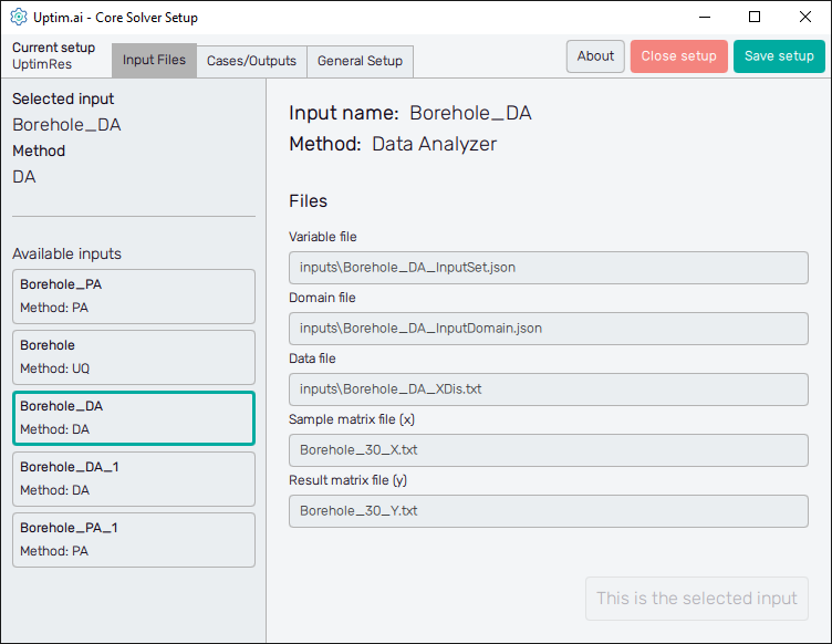
Figure 1 shows the initial screen of the Core Solver Setup GUI. The strip on the top of the window is common for all methods. From the left, at first, it informs the user about the setup file which is being processed. Then, there are three tabs of solver settings:
- Input Files : Here the user selects the set of inputs to be used and sees the list of corresponding files
- Cases/Outputs : The setup for the selected method and each solver run
- General Setup : The user can define the names of model result files as well as computational resources reserved for the Uptimai Solver
The control panel on top then continues with the About button with the menu dedicated to
accessing the link to this document (Help), contacting Uptimai company to get the support
(Company), and showing the information about the currently installed version of the
program (Version). The Close button ends the preparation of the current setup (also with
the option to discard the data), and the Save setup button stores all changes into the
*.json file. Also, there are ? icons on the solver setting tabs to show
quick reference to the corresponding entry field or feature.
Input Files#
The left section of the screen contains the general information about the Selected input. There is its name together with the Method to be used in the Uptimai Solver (in this case the Data Analysis) that was identified automatically from files of the selected input. The user can change the set of inputs (together with the method, eventually) from the list of Available items below.
When going through the list of available sets of inputs, the program shows their details in the right section of the GUI window. To choose a particular set of inputs as the currently selected one, double-clicking or confirmation with the Select this input button is required. When the reviewed input is the selected one, the aforementioned button is disabled and informs the user that This is the selected input.
Cases/Outputs#
Here the user defines solver options for all cases in the current setup. Cases are listed in the left section of the program window, as seen in Figure 2. It is possible as many cases as needed, the Uptimai Solver will process them in the order prescribed by the list. The position of each case in the list can be changed by ist mouse-dragging by its = symbol. Clicking the X icon of the item will remove the case from the list. Other cases can be added to the list via the + Add case below the list.
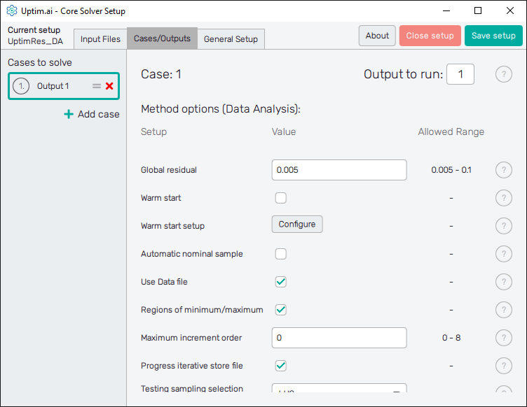
Cases in the list have generic names based on the project output which should be solved in the model. Clicking a list item highlights it in the list and the corresponding individual settings are shown in the right section of the window. The corresponding case number can be seen also on top of the right section of the GUI to ensure users with on which case they work. The top of the right section also contains the entry field where the Output to run is set. In other words, it is the column of the result matrix to be evaluated by the Uptimai solver.
Number of outputs
The Uptimai solver checks automatically the total number of outputs in the matrix of results by counting the number of columns. Be sure you are not calling the output number out of the existing range of columns in the matrix of results!
In the Method options below is the list of Setup entry fields, drop-down menus, or switches that are available for the Data Analysis method. Each entry field Value has to comply with the prescribed Allowed range. Options to be set are:
Global residual : This number represents the relative residual, which is set for the mean value of the variance of results. The algorithm iterates until the residual is achieved for both observed values, i.e.: the mean value and the variance.
Warm start : Enables incremental learning by using matrices X and Y enhanced with new samples together with an existing
*.upstresult file. Be aware of the need for the full compatibility of all input files with the*.upstfile and its corresponding setup*.jsonused for this previous run.Warm start setup : The Configure button opens the separate dialogue window with options for the Warm start. The
*.upstfile to be enhanced with additional samples is selected and confirmed here.Automatic nominal sample : Allows computing the position of the nominal sample for the surrogate as the centre of the matrix of samples. Otherwise, the nominal sample defined in the preprocessor will be used.
Use data file
Enables propagation of output values for all Monte-Carlo samples defined in the input domain distributions. Allowing this option is required for the analysis of the stochastic model of the solved problem in the Uptimai Postprocess tool. Otherwise, only the interpolation of model outputs can be used.Regions of minimum/maximum : Enables Regions of minimum/maximum to be computed. This process takes place at the end of each Uptimai Solver run. With this option off, the Regions of minimum/maximum feature is not available for the postprocess.
Maximum increment order : The maximum increment order sets the maximum allowed order of increment functions included in the model for purposes of visualization and postprocess. Unlike the Uncertainty Quantification method, the precision of the trained model is not affected by this setting. Restricting the order of increment may speed up the model-building process, especially for problems with a large number of input variables. Although the statistical analysis of variables will be identical, details of increment functions will not be available for higher-order increment functions (including the Sensitivity Analysis)
The maximum increment order to be set is limited to 3 because of the inability to display increments of higher order. Setting the value to 0 will use the highest possible increment for display.
Progress iterative store file : Enables storing the current progress of the learning algorithm, which can be restored in case of an unexpected collapse of the code. Loading the progress from a file may significantly decrease the overall wall-clock time of the repeated learning process. The progress iterative store file needs to be fully compatible with the project and the current solver settings!
OLD FILES
The file is stored under a generic name Progress_iterative_store_file_Ox_Cx.prog that
only differentiates the number of the output and its position in the sequence of
cases to be solved.
The existing progress iterative file has to be deleted when the settings of the learning
process are changed. Uptimai Solver will not proceed from the progress iterative file
which is incompatible with the current setup!
Testing sampling selection scheme : The Testing sampling selection scheme controls the distribution of samples used for the testing and validation of the model. Available options are:
- Latin Hypercube Sampling (LHS) : Spreads testing samples uniformly
along the domain to cover the design space evenly. Tuned for the polynomial trend functions and especially useful for small data sets. It is suitable for most problems in general. - Distance : Prefers testing samples on boundaries of the domain, and thus it is suited for the stabilization of the model on the boundaries and later prediction outside the domain. Tuned for the polynomial trend function.
- Random : Selects samples randomly and should be used for large datasets only, where the precision is not affected and there is a significant speed-up in comparison with other sampling schemes.
- Data input : Users can call for their own set of samples that are different from samples used for training of the model. Files with samples for testing are defined in section Testing sampling selection scheme input under the Configure button.
- Clustered : Selects the validation samples in clustered regions, i.e. the validation samples are clustered in certain parts of the domain. The cluster centres are randomly selected around the domain.
- Latin Hypercube Sampling (LHS) : Spreads testing samples uniformly
Testing sampling selection scheme input : The Configure button opens the separate dialogue window with options for the Testing sampling selection scheme. Available options are:
- Test matrix samples (x) : Path to
*.txtfile with matrix of comma separated values of input variables of samples selected for testing and validation. - Test matrix results (y) : Path to
*.txtfile with matrix of comma separated output values of samples selected for testing and validation. - Max # of samples : Maximum number of test samples to be used from the matrix of test samples in case it is larger. Samples are selected randomly from the matrix.
- Test matrix samples (x) : Path to
Smooth learner depth : The smoothing model is built over the top of the polynomial trend function. It helps to tacle discontinued behavior and deviations from the general trend.
- None : No smoothing model is used.
- Main : Uses only the main model on the level of variables and doesn't dive into sub-models. Suitable for initial training and if speed is preferred.
- Full : This scheme splits the domain into smaller domains to crete set of additional sub-models. The best combination of sub-models is selected to increase the overall accuracy. slower than the Main option, but it can improve the accuracy, especially if there is a small number of samples.
Random state : The random state seed used for the learning process.
Trend model : Turns on the creation of the basic trend polynomial model, that can be combined with the smooth learner. Ideal for small data sets to establish the basic relationships between inputs and output values.
Enhanced model : Using the Enhanced model splits the domain into set of smaller domains and builds the polynomial model for each of these. Increases the accuracy of the Trend model option but increases computational time. Applicable only with the Trend model on!
Preprocessor sample threshold : Maximum number of samples to be used for training. Applied only if the switch is on and the loaded matrix of training samples is larger.
Preprocessor sample threshold type : If a large data set is passed to the training process and the speed of the learning needs to be accelerated, it selects only a small portion of samples based on the selected criteria.
- None : Do not use the preprocessing of the set of samples.
- Random : Samples are selected randomly.
- K-means : Reduce the number of samples to centres of k-means. Suited for problems with clustered input data where simplifications are necessary.
- Random select : Randomly selects the required number of samples for both training and testing so the total number of samples included is defined by the threshold. However, in the postprocessing phase, a full dataset is used, i.e. the user sees all samples loaded from the file.
- Random weighted : Randomly (uniform probability) selects the samples on the Y abscissa according to the number of selected bins, i.e. samples are selected based on their values. It is useful if the function consists of a large number of the same values with small peaks - small peaks are selected and large areas with the same samples are only sparsely selected. It ensures the full spectrum of output values is represented in the set of samples.
Learner type : Select type of the smoothing model. Currently Gaussian process, Multi-Layer Perceptron (MLP), Light Gradient-Boosting Machine (LightGBM), and Gradient Boosting framework mod XGBoost are available.
Learner type (sub-model) : Select type of sub-functions of the smoothing model. Currently Gaussian process, Multi-Layer Perceptron (MLP), Light Gradient-Boosting Machine (LightGBM), and Gradient Boosting framework mod XGBoost are available.
Sub-model nonzero assumption : It is connected to the evaluation of sub-models. If turned off (default value), it assumes that the error of the main model has a Gaussian distribution. If turned on, the distribution of errors is non-gaussian.
Especially if the nominal sample is in the centre of the domain, enabling this option brings additional accuracy. However, it is case-specific. Also, this option has to be false for the incremental learning /- Warm start.
General Setup#
The management of project results files and computer resources reserved for the Uptimai Solver is defined in the General setup tab.
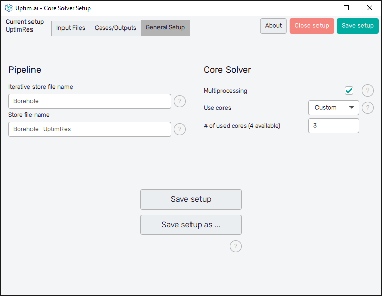
In the Pipeline section on the left can the user adjust the names of files where all results
received from the solver run are stored. Iterative store file name sets the prefix for
the *.itr file which holds data values of all samples already collected from a
third-party software. The Data Analysis does not use this file, therefore this option
remains disabled.
Store file name sets the naming convention for the final resulting file produced by the
Uptimai Solver. This *.upst contains the set of statistical results
suitable for analysis in the Uptimai Postprocessor.
The default basename is proposed as the <project_name> followed
by the <setup-file_name>, the number of the output being solved, and the number
of the currently processed case. For reference, see the default name of the result file of the
project shown in Figure 3, where the second output was solved as the first case
according to the solver setup:
Borehole_UptimRes_O2_C1.upst
The name of the *.upsi file with the surrogate model suitable for processing through the
separate Interpolant tool is composed in the same way.
The main goal of the proposed convention is to give a hint to the user on how to match the project
files with particular settings of the Uptimai Solver just from the look into the file explorer.
The Core Solver section on the right of the window is about the number of CPU cores used by the Uptimai Solver when working. The Multiprocessing switch allows more than one core to be used in the first place. In such cases, the Use cores drop-down menu is enabled where the user can specify the number of cores dedicated to the Uptimai Solver. Besides arbitrary setting the Custom number of cores to be used in a separate entry field, there are two other options in the menu. All allows the solver to use all cores present in the system, while the All-1 option leaves one additional core free for other tasks. The suggested approach is to choose All-1 by default.
The Save setup button at the bottom of the GUI window saves the current setup directly under the existing name into the project directory. The button Save setup as ... opens the file dialogue allowing the user to change the file name and the path of the setup file.