Direct Optimization
Uptimai Direct Optimization gives the optimum of a given problem. Unlike the Statistical Optimization approach, it does not build any intermediate surrogate models — instead, it directly explores the design space using robust, well-established optimization algorithms such as Differential Evolution (DE), CMA-ES, Nelder-Mead, and GSS.
To further increase efficiency, the method applies a function decoupling strategy, where the problem is intelligently separated into smaller, lower-dimensional subproblems that can be solved independently. This significantly reduces the number of required samples while maintaining high accuracy in the search for the optimum. Moreover, in high-dimensional spaces, it tends to reach higher-quality optima than simple optimizers.
The Direct Optimization method running in the "Function call" mode will call for outputs corresponding to specific combinations of input parameters, thus, it is intended for work in connection with engineering computational codes etc.
How to use the interface
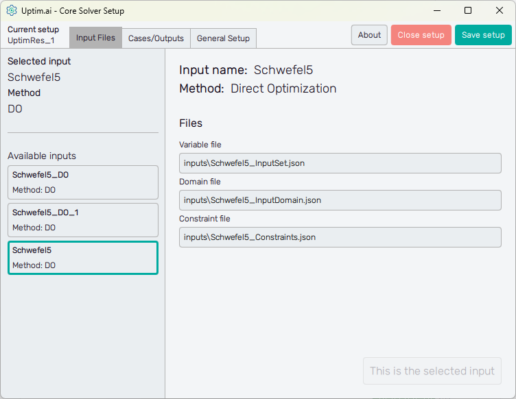
Figure 1 shows the initial screen of the Core Solver Setup GUI. The strip on the top of the window is common for all methods. From the left, at first, it informs the user about the setup file which is being processed. Then, there are three tabs of solver settings:
- Input Files : Here the user selects the set of inputs to be used and sees the list of corresponding files
- Cases/Outputs : The setup for the selected method and each solver run
- General Setup : The user can define the names of model result files as well as computational resources reserved for the Uptimai Solver
The control panel on top then continues with the About button with the menu dedicated to
accessing the link to this document (Help), contacting Uptimai company to get the support
(Company), and showing the information about the currently installed version of the
program (Version). The Close button ends the preparation of the current setup (also includes
the option to discard the data), and the Save setup button stores all changes to the
*.json file. Also, there are ? icons on the solver setting tabs to show
quick reference to the corresponding entry field or feature.
Input Files
The left section of the screen contains the general information about the Selected input. There is its name together with the Method to be used in the Uptimai Solver (in this case the Direct Optimization) that was identified automatically from files of the selected input. Users can change the set of inputs (together with the method, eventually) from the list of Available inputs below.
When going through the list of available sets of inputs, the program shows their details in the right section of the GUI window. To choose a particular set of inputs as the currently selected one, double-clicking or confirmation with the Select this input button is required. When the reviewed input is the selected one, the aforementioned button is disabled and informs the user that This is the selected input.
Cases/Outputs
Here the user defines solver options for all cases in the current setup. Cases are listed in the left section of the program window, as seen in Figure 2. It is possible as many cases as needed, the Uptimai Solver will process them in the order prescribed by the list. The position of each case in the list can be changed by ist mouse-dragging by its = symbol. Clicking the X icon of the item will remove the case from the list. Other cases can be added to the list via the + Add case below the list.
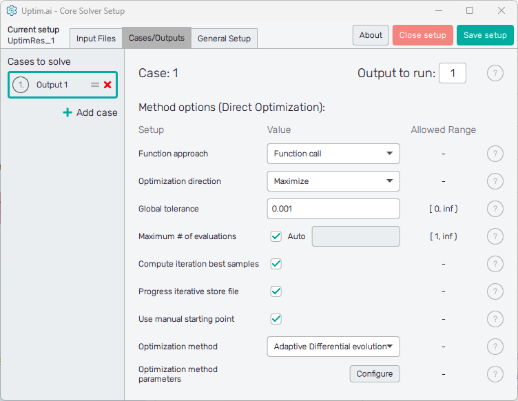
Cases in the list have generic names based on the project output which should be solved in the model. Clicking a list item highlights it in the list and the corresponding individual settings are shown in the right section of the window. The corresponding case number can be seen also on top of the right section of the GUI to ensure users with on which case they work. The top of the right section also contains the entry field where the Output to run is set. In other words, it is the column of the result matrix to be evaluated by the Uptimai solver.
The Uptimai solver checks automatically the total number of outputs in the matrix of results by counting the number of columns. Be sure you are not calling the output number out of the existing range of columns in the matrix of results!
In the Method options below is the list of Setup entry fields, drop-down menus, or switches that are available for the Direct Optimization method. Each entry field Value has to comply with the prescribed Allowed range. Options to be set are:
- Function approach
: Which approach is used for the optimization process sampling.
- Function call - An actual function that will be used to evaluate samples using the coupling mechanism.
- Data model - Precomputed surrogate model created using the Data Analysis method will be used to evaluate samples.
- Function approach parameters
: In case the 'Function call' approach is selected, there is nothing to configure. In case the 'Data model' approach is selected, there is one additional parameter:
- Model file - Path to the surrogate model file created using the Uptimai Data Analysis or Uncertainty Quantification method. The file must be compatible with the selected input:
- Matching variable count, names, distribution types with their parameters.
- If the model contains variable with distribution types Data driven, Data driven (discrete) or Data driven (boolean) and if the setup contains multiple cases using the 'Data model' approach, all models must reference the same "Matrix_X" file (stored inside the .upsi file), as this matrix is effectively a parameter of the distribution type in such case.
- Model file - Path to the surrogate model file created using the Uptimai Data Analysis or Uncertainty Quantification method. The file must be compatible with the selected input:
- Optimization direction : The direction of the optimization shows if the optimization has to maximize (find the area with maximum output values) or minimize (find the area with minimum output values).
- Tolerance : Threshold that will stop the optimization process, if the convergence rate drops below the value specified.
- Maximum # of evaluations : Maximum number of function evaluations allowed. The optimization process will stop, if the number of evaluations defined is reached. Note that the solver can request an additional small number of samples beyond this threshold, to evaluate the final population of samples, especially if the 'Compute iteration best samples' option is enabled. If set to 'auto', the value will be computed based on the dimension of the problem. The exact formula is the following (d is the dimensionality of the problem, i.e. the number of variables):
- Compute iteration best samples : If enabled, the best known sample from each iteration will be evaluated. This will be done after the optimization process is finished, in a single batch.\n\nIf disabled, those samples will not be evaluated to save unnecessary function evaluations, as this is useful only for postprocessing and has no effect on the optimization process and its result. If disabled, the 'Iterations overview' section will not be available in the Postprocessor.
- Progress iterative store file
: Enables storing the current progress of the learning algorithm, which can be restored in the case of an
unexpected collapse of the code.
note
Please delete the progress iterative file when changing the case settings. Uptimai solver will not proceed from the progress iterative file which is incompatible with the settings.
- Use manual starting point : If enabled, the starting point defined in the domain file will be used. If disabled, the middle of the interval will be used.
- Optimization method
: The optimization method to use:
- Differential evolution - The standard implementation of the Differential Evolution algorithm.
- Differential evolution (decoupled) - The function is decoupled into multiple smaller sub-problems, which are then optimized using the Differential Evolution algorithm.
- Adaptive Differential evolution - Same as the 'Differential evolution (decoupled)', but the decoupling is done multiple times throughout the optimization process, depending on other parameters.
- Hybrid CMA-DE - The function is decoupled into multiple smaller sub-problems, which are then optimized using the CMA-ES algorithm (N-D sub-problems) or the Differential Evolution (1-D sub-problems).
- Adaptive Hybrid CMA-DE - Same as the 'Hybrid CMA-DE', but the decoupling is done multiple times throughout the optimization process, depending on other parameters.
- Hybrid NM-GS - The function is decoupled into multiple smaller sub-problems, which are then optimized using the Nelder-Mead algorithm (N-D sub-problems) or the Golden-Section Search algorithm (1-D sub-problems).
note
Note that both Nelder-Mead and Golden-Section Search assume the optimized function is unimodal. In case the decoupled sub-problems are multimodal, this method may identify local rather than global extrema.
- Adaptive Hybrid NM-GS - Same as the 'Hybrid NM-GS', but the decoupling is done multiple times throughout the optimization process, depending on other parameters.
- Optimization method parameters : Parameters of the individual optimization methods are described in the subsections below
Differential evolution
- Population size multiplier : The population size of the optimizer is directly proportional to the selected value, along with the dimensionality of the problem. Larger values increase exploration and robustness but also raise the computational cost.
- Mutation constant : Controls the scale of differential variation applied during mutation (typically between 0.4 and 1.0). Higher values promote exploration by making larger jumps in the search space, while lower values focus the search around existing solutions.
- Crossover probability : Specifies the likelihood (between 0 and 1) that parameters from the mutated candidate will replace those in the current individual. A higher probability encourages greater diversity and exploration; a lower one preserves more of the parent’s characteristics.
Differential evolution (decoupled)
- # of decoupling test points : The number of test points used by the decoupling process. The number of samples required by the decoupling process has a linear relationship with this value and the dimensionality of the problem. Higher values increase the precision of the decoupling process at the cost of additional sample evaluations.
- Tolerance for decoupling : This option controls how strong the interaction between variables need to be to prevent decoupling. Lower values lead to a more restricted decoupling process, higher values allow for a more flexible one (less constrained), potentially improving performance at the expense of accuracy.
- Population size multiplier : The population size of the optimizer is directly proportional to the selected value, along with the dimensionality of the decoupled sub-problems. Larger values increase exploration and robustness but also raise the computational cost.
- Mutation constant : Controls the scale of differential variation applied during mutation (typically between 0.4 and 1.0). Higher values promote exploration by making larger jumps in the search space, while lower values focus the search around existing solutions.
- Crossover probability : Specifies the likelihood (between 0 and 1) that parameters from the mutated candidate will replace those in the current individual. A higher probability encourages greater diversity and exploration; a lower one preserves more of the parent’s characteristics.
Adaptive Differential evolution
- # of decoupling test points : The number of test points used by the decoupling process. The number of samples required by the decoupling process has a linear relationship with this value and the dimensionality of the problem. Higher values increase the precision of the decoupling process at the cost of additional sample evaluations.
- Tolerance for decoupling : This option controls how strong the interaction between variables need to be to prevent decoupling. Lower values lead to a more restricted decoupling process, higher values allow for a more flexible one (less constrained), potentially improving performance at the expense of accuracy.
- Population size multiplier : The population size of the optimizer is directly proportional to the selected value, along with the dimensionality of the decoupled sub-problems. Larger values increase exploration and robustness but also raise the computational cost.
- Mutation constant : Controls the scale of differential variation applied during mutation (typically between 0.4 and 1.0). Higher values promote exploration by making larger jumps in the search space, while lower values focus the search around existing solutions.
- Crossover probability : Specifies the likelihood (between 0 and 1) that parameters from the mutated candidate will replace those in the current individual. A higher probability encourages greater diversity and exploration; a lower one preserves more of the parent’s characteristics. Adaptive scheme
- Adaptive scheme
: How the adaptive scheme determines when a new decoupling attempt should be made:
- Auto - the decoupling attempts are triggered by the rate of shrinking of the envelope of the current population.
- Fixed step - the decoupling attempts are triggered by the number of iterations performed.
- Adaptive scheme parameters : Parameters of the adaptive scheme are common for all adaptive methods and are described in a separate subsection.
Hybrid CMA-DE
- # of decoupling test points : The number of test points used by the decoupling process. The number of samples required by the decoupling process has a linear relationship with this value and the dimensionality of the problem. Higher values increase the precision of the decoupling process at the cost of additional sample evaluations.
- Tolerance for decoupling : This option controls how strong the interaction between variables need to be to prevent decoupling. Lower values lead to a more restricted decoupling process, higher values allow for a more flexible one (less constrained), potentially improving performance at the expense of accuracy.
- Population size multiplier : The population size of the optimizer is directly proportional to the selected value, along with the dimensionality of the decoupled sub-problems. Larger values increase exploration and robustness but also raise the computational cost.
- Mutation constant : Controls the scale of differential variation applied during mutation (typically between 0.4 and 1.0). Higher values promote exploration by making larger jumps in the search space, while lower values focus the search around existing solutions.
- Crossover probability : Specifies the likelihood (between 0 and 1) that parameters from the mutated candidate will replace those in the current individual. A higher probability encourages greater diversity and exploration; a lower one preserves more of the parent’s characteristics.
- Initial covariance step size : Specifies the initial standard deviation of the sampling distribution used to generate candidate solutions for the CMA-ES optimizers. It defines the starting search radius around the initial mean — larger values enable broader exploration of the search space, while smaller values focus the search locally near the starting point.
Adaptive Hybrid CMA-DE
- # of decoupling test points : The number of test points used by the decoupling process. The number of samples required by the decoupling process has a linear relationship with this value and the dimensionality of the problem. Higher values increase the precision of the decoupling process at the cost of additional sample evaluations.
- Tolerance for decoupling : This option controls how strong the interaction between variables need to be to prevent decoupling. Lower values lead to a more restricted decoupling process, higher values allow for a more flexible one (less constrained), potentially improving performance at the expense of accuracy.
- Population size multiplier : The population size of the optimizer is directly proportional to the selected value, along with the dimensionality of the decoupled sub-problems. Larger values increase exploration and robustness but also raise the computational cost.
- Mutation constant : Controls the scale of differential variation applied during mutation (typically between 0.4 and 1.0). Higher values promote exploration by making larger jumps in the search space, while lower values focus the search around existing solutions.
- Crossover probability : Specifies the likelihood (between 0 and 1) that parameters from the mutated candidate will replace those in the current individual. A higher probability encourages greater diversity and exploration; a lower one preserves more of the parent’s characteristics.
- Initial covariance step size : Specifies the initial standard deviation of the sampling distribution used to generate candidate solutions for the CMA-ES optimizers. It defines the starting search radius around the initial mean — larger values enable broader exploration of the search space, while smaller values focus the search locally near the starting point.
- Adaptive scheme
: How the adaptive scheme determines when a new decoupling attempt should be made:
- Auto - the decoupling attempts are triggered by the rate of shrinking of the envelope of the current population.
- Fixed step - the decoupling attempts are triggered by the number of iterations performed.
- Adaptive scheme parameters : Parameters of the adaptive scheme are common for all adaptive methods and are described in a separate subsection.
Hybrid NM-GS
- # of decoupling test points : The number of test points used by the decoupling process. The number of samples required by the decoupling process has a linear relationship with this value and the dimensionality of the problem. Higher values increase the precision of the decoupling process at the cost of additional sample evaluations.
- Tolerance for decoupling : This option controls how strong the interaction between variables need to be to prevent decoupling. Lower values lead to a more restricted decoupling process, higher values allow for a more flexible one (less constrained), potentially improving performance at the expense of accuracy.
Adaptive Hybrid NM-GS
- # of decoupling test points : The number of test points used by the decoupling process. The number of samples required by the decoupling process has a linear relationship with this value and the dimensionality of the problem. Higher values increase the precision of the decoupling process at the cost of additional sample evaluations.
- Tolerance for decoupling : This option controls how strong the interaction between variables need to be to prevent decoupling. Lower values lead to a more restricted decoupling process, higher values allow for a more flexible one (less constrained), potentially improving performance at the expense of accuracy.
- Adaptive scheme
: How the adaptive scheme determines when a new decoupling attempt should be made:
- Auto - the decoupling attempts are triggered by the rate of shrinking of the envelope of the current population.
- Fixed step - the decoupling attempts are triggered by the number of iterations performed.
- Adaptive scheme parameters : Parameters of the adaptive scheme are common for all adaptive methods and are described in a separate subsection.
Adaptive scheme parameters
-
Early stop threshold : The threshold which will stop the additional decoupling attempts to save sample evaluations required by the decoupling process. When the function is decoupled so that the maximum dimension of a sub-problem is lower or equal to the selected value, no additional decoupling attempts will be made.
noteNote that setting this to 0 will effectively disable this mechanism, making the occurrence of the decoupling attempts depend solely on the other adaptive scheme parameters.
Setting this to a value greater or equal to the number of input variables will effectively transform the selected adaptive optimization method to its non-adaptive counterpart (the decoupling will be done only once, at the beginning of the optimization process).
-
Bounds reduction factor (only for Adaptive scheme: Auto) : A new decoupling attempt is triggered, when the geometric mean of the ratios of interval lengths in each dimension of the current population to the interval lengths in each dimension of the population at the point of the previous decoupling attempt drops below the selected value.
-
# of iterations per step (only for Adaptive scheme: Fixed step) : A new decoupling attempt is triggered each time the selected number of iterations is performed.
noteThis can vary slightly for the 'Adaptive NM-GS' optimization method, as the Nelder-Mead optimizers may require up to two additional iterations before they can be interrupted.
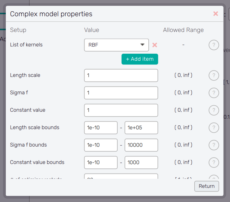
Configure window
Separate windows with configuration options are accessible with the Configure button. This button typically appears together with a menu item which requires detailed configuration. Window appearance and the list of options is changing according the item being configured. The help is available for each option item via the ? button next to it. The Configure button can also appear in the configure window itself, opening its another layer.
The setup of the configure window is confirmed with the Return button, which also brings the user back to the previous screen.
General Setup
The management of project results files and computer resources reserved for the Uptimai Solver is defined in the General setup tab.
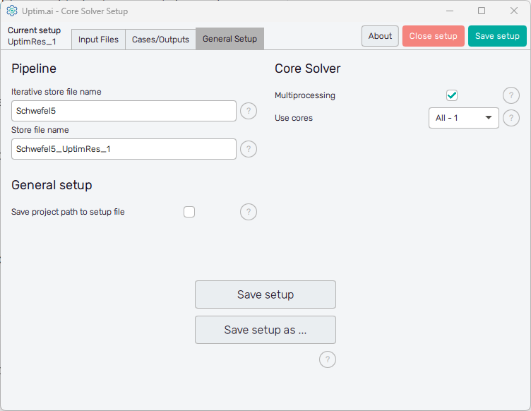
In the Pipeline section on the left can the user adjust the names of files where all results
received from the solver run are stored. Iterative store file name sets the prefix for
the *.itr file which holds data values of all samples already collected from a
third-party software. The default basename is set as <project_name>.
Store file name sets the naming convention for the final resulting file produced by the
Uptimai Solver. This *.upst contains the set of statistical results
suitable for analysis in the Uptimai Postprocessor.
The default basename is proposed as the <project_name> followed
by the <setup-file_name>, the number of the output being solved, and the number
of the currently processed case. For reference, see the default name of the result file of the
project shown in Figure 3, where the first output was solved as the first case
according to the solver setup:
Schwefel5_UptimRes_1_O1_C1.upst
The Core Solver section on the right of the window is about the number of CPU cores used by the Uptimai Solver when working. The Multiprocessing switch allows more than one core to be used in the first place. In such cases, the Use cores drop-down menu is enabled where the user can specify the number of cores dedicated to the Uptimai Solver. Besides arbitrary setting the Custom number of cores to be used in a separate entry field, there are two other options in the menu. All allows the solver to use all cores present in the system, while the All-1 option leaves one additional core free for other tasks. The suggested approach is to choose All-1 by default.
The Save setup button at the bottom of the GUI window saves the current setup directly under the existing name into the project directory. The button Save setup as ... opens the file dialogue allowing the user to change the file name and the path of the setup file.