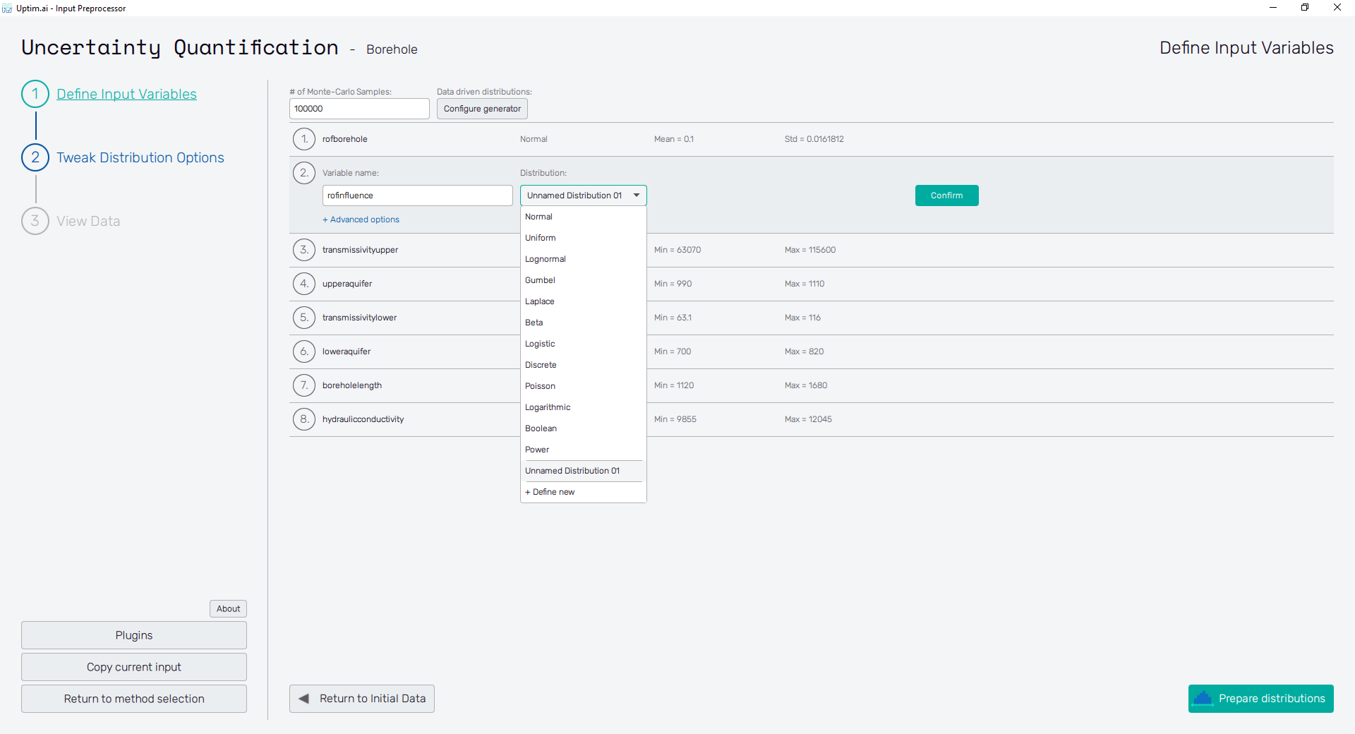
Input distribution types
When defining the design space of the project, the user needs to decide not only the range of values for each input distribution but also its probability distribution. Especially for variables representing e.g. environmental variables or material characteristics, this allows to setup of the case to be much closer to real-world conditions. As a result, the obtained mathematical model represents the reality in a better way.
Featured distribution types
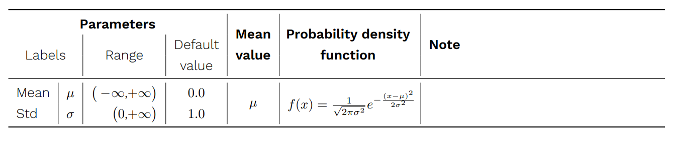
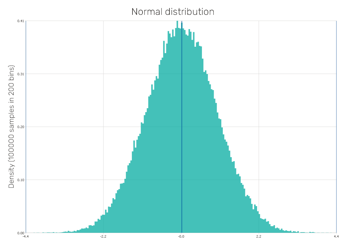
Normal distribution
Normal distribution, also known as Gaussian distribution, is a continuous probability distribution that is symmetric around its mean value. According to the empirical rule, 99.7% of all its values lie within three standard deviations of the mean value. It is expected for physical quantities that are a sum of many independent processes affected by random errors, e.g. material properties.
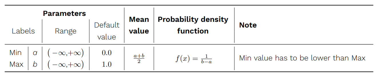
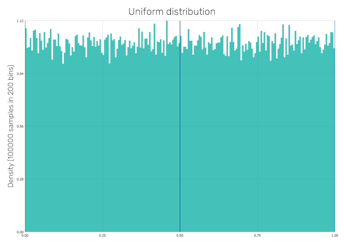
Uniform distribution
It is considered a continuous symmetric distribution where the probability of occurrence in the distribution is equal for all values from a given range. It is a type of distribution well-suited for all input parameters dependent on the designer's decision.
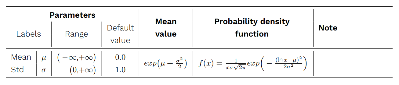
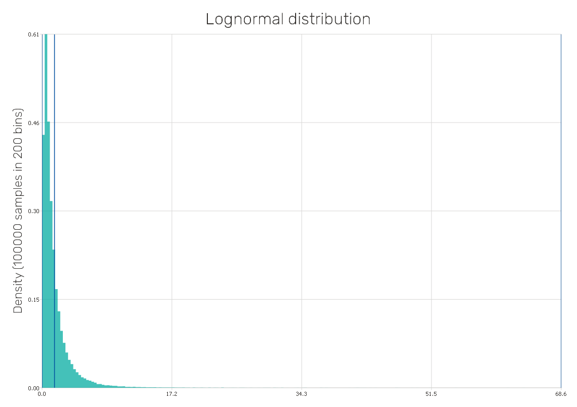
Lognormal distribution
It is a continuous probability distribution where the logarithm of its values is distributed normally. This distribution consists of real positive values only. It can be observed among various phenomena in the fields of e.g. biology, sociology, chemistry, technology, and finance.
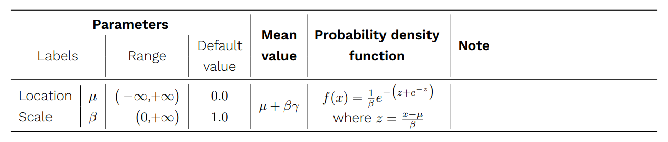
Gumbel distribution
It is a continuous distribution describing the distribution of the maximum (or the minimum) values of a series of distributions, e.g. maximum rainfall rate in a series of distributions measured over time. Since it is related to the duration of time up to an event, its use can be in e.g. reliability analysis in engineering.

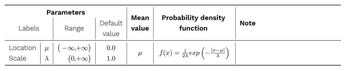
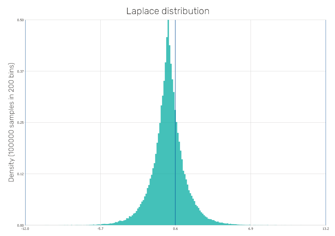
Laplace distribution
It is a symmetric continuous probability distribution also known as the double exponential distribution, since it can be seen as an exponential distribution mirrored around the location parameter. It is the distribution of differences between two independent varieties with identical exponential distributions. It can be used for describing the distribution of errors in observed values.
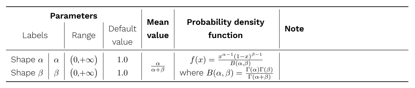
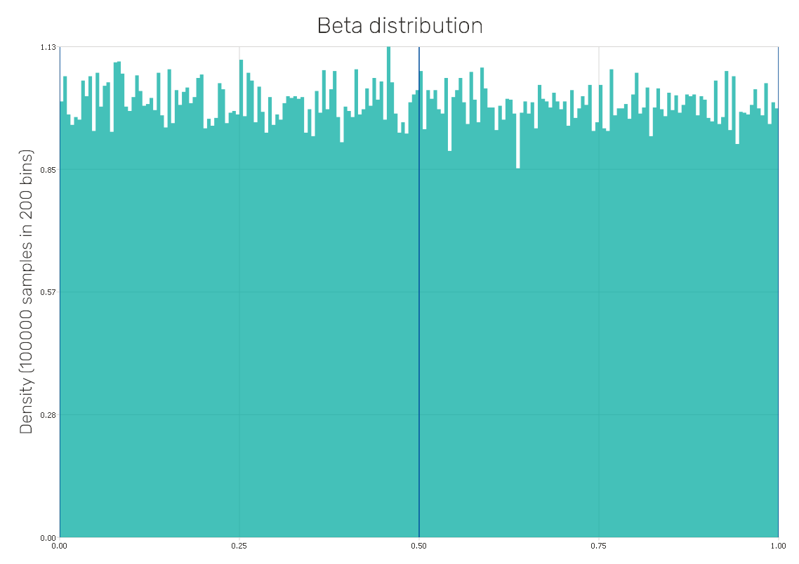
Beta distribution
It is a continuous probability distribution defined on the interval (0,1), thus, it can be used to model random variables of prescribed length. Settings of its two parameters can result in a wide variety of shapes of the distribution (e.g. it turns out to be the uniform distribution with default values of parameters, same as in Figure 2), therefore, there is a wide variety of its use.
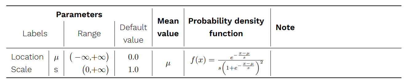
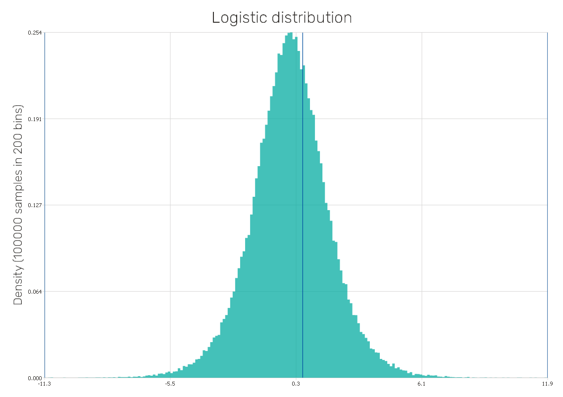
Logistic distribution
It is a symmetric continuous probability distribution very similar to the normal distribution in its appearance but has heavier tails, which can increase the robustness of analyses based on it when compared to those using the normal distribution. It is used for logistic regression model predicting the likelihood of an event based on an input variable.
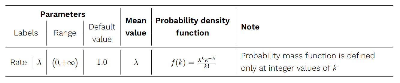
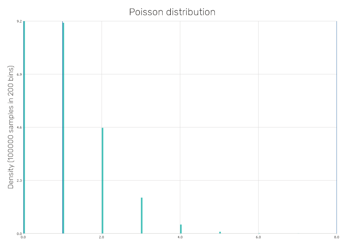
Poisson distribution
It is a discrete probability distribution used to represent integer-valued counts, such as the number of events observed within an interval of time or other specified dimensions such as distance, area or volume. Therefore, it is used for applications in many fields related to counting individual objects, e.g. astronomy, biology, and telecommunication.
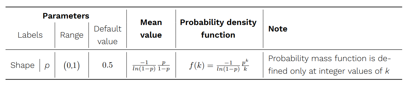
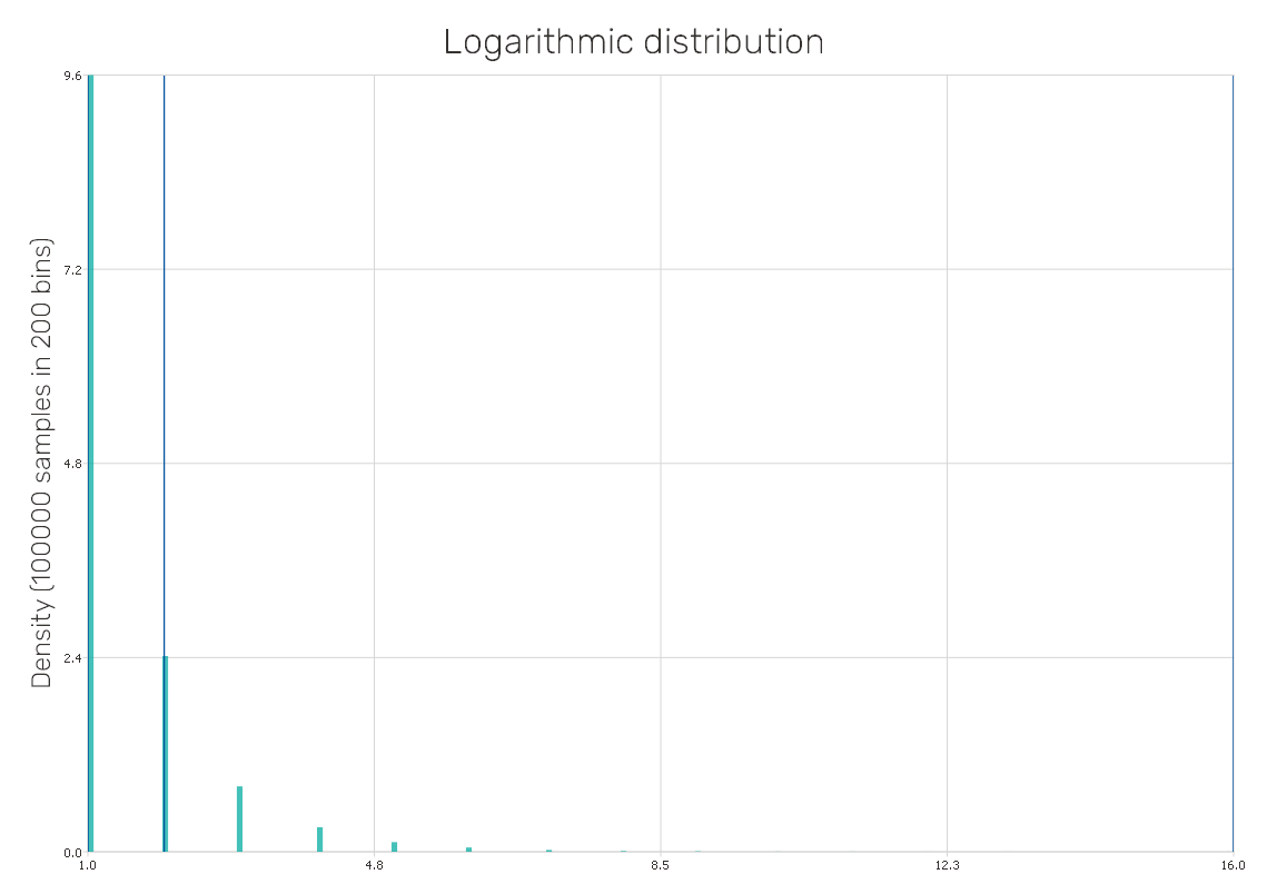
Logarithmic distribution
Also known as the logarithmic series distribution, is a discrete probability distribution based on the standard power series expansion of the natural logarithm function. It can be used in cases involving several event occurrences within a time period or space.
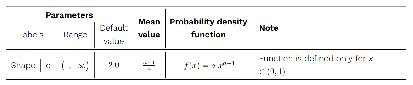
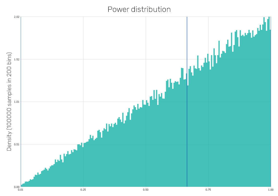
Power distribution
It is a continuous probability distribution defined on the interval (0,1), also known as the power function distribution. It also may be seen as the inverse of the Pareto distribution, thus, its application can cover a similar range of problems.
Discrete distribution
As the name suggests, it is a discrete type of distribution, in this case completely arbitrary according to the user's needs. As inputs, two vectors of comma-separated values are required. One is the Vector of positions setting distribution values, the other is the Vector of weights setting ratios of values in the input distributions. At least three distinct position values must be given, weights must be greater than zero.
Boolean distribution
A special case of the discrete distribution. Although in its traditional meaning it is used as a or value switch, here it is not limited so strictly. In general, it can be used for any parameter splitting data into two categories. To define the distribution, the user only needs to enter two position values (i.e. categories, characteristics, limits, etc.) and their weights. As for the regular discrete distributions, weights have to be greater than zero.
Data-driven distributions
When dealing with the Data Analysis method, it might be required to work with distributions as close as possible to those of training data in a loaded X matrix. Therefore, input distributions respecting the loaded data are possible to be created. In principle, the loaded data is split into clusters in the first step and then these clusters are populated according to the selected rule. Distributions of samples are created according to the setup that can be found under the Configure generator button at the top of the screen:
- Type of local sampling : Distribution type used for the sampling around the center of each cluster.
- # of clusters coef. : The coefficient used for the computation of the total number of clusters. The number of clusters affects their diameter and thus the spread of samples across the domain. The higher number of clusters results in distributions with more distinct edges and more concentrated around loaded samples.
There are also sub-variants of this type of distribution dealing with discrete or boolean samples if the solved problem requires these. The configuration setup of created distributions remains the same. However, the selected distribution type allows only values already included in the source data to be included in the distribution.
User defined distribution
The principle is similar to the discrete distribution, but this custom set distribution is continuous. Its parameters are set through a standalone GUI whose features are described in a separate sheet available with the Distribution Creator tool described below.
Distribution Creator
With the help of the Distribution Creator, a distribution of an
arbitrary shape according to the user's needs can be prepared. It is an
add-on of the Input Preprocessor program popping up on + Define new
item selection from the distribution selector. The distribution shape is designed directly in the
graphic interface allowing one to see the resulting shape immediately.
The distribution shape itself can be also loaded from a *.csv file when needed.
How to use the interface
The initial state of the application's window can be seen in
Figure 11. On the left, there is the Existing custom distributions
section, where the management of user defined distributions present in the project can be done.
By clicking on items in the list below the user can either Edit the existing distribution
or Make a copy of it, which can be renamed and adjusted separately. Below the list, there are two
buttons. Create new starts a new distribution preparation from scratch. The button Load form
data file allows users to upload coordinates of the distribution's control points directly from a
*.csv file. It is a very useful option for situations where the probability distribution can be
e.g. measured or found in the literature. The source file needs to have two comma-separated
columns defining X and Y coordinates of control points. This formatting is very similar to what the
user can see in the GUI when creating the distribution directly in the tool.
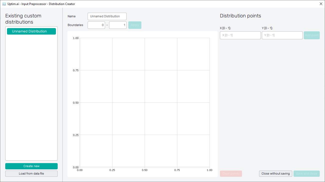
The central section of the GUI window is dedicated to the graphical definition of the input distribution. On the top of this section, there is an entry field where the input distribution name can be changed. This modification appears instantly in the list on the left. Be aware that the name of each input distribution has to be unique. Right under the Name entry, the Boundaries of the input distribution shape can be adjusted. It is the setting of limits applicable for all definition points of the distribution, it is not possible to create a definition point outside the boundaries.
There are two possibilities for how to handle definition points in case of restricting/cropping boundaries of an existing distribution shape. First, points not fitting into cropped boundaries can be deleted completely. The second option is to scale the whole distribution based on the new range of boundaries.
The gridded canvas making the most of the area is an interactive space for the definition of the input distribution shape. Just by the left mouse button clicking, the user can create new definition points of the input distribution shapes - their position within the boundaries and the weight of each point ranging from 0 to 1. Unwanted definition points can be easily removed by the right mouse button click at these. Dragging a point with the mouse adjusts its position and weight but with the restriction given by distribution boundaries and/or positions of surrounding definition points.
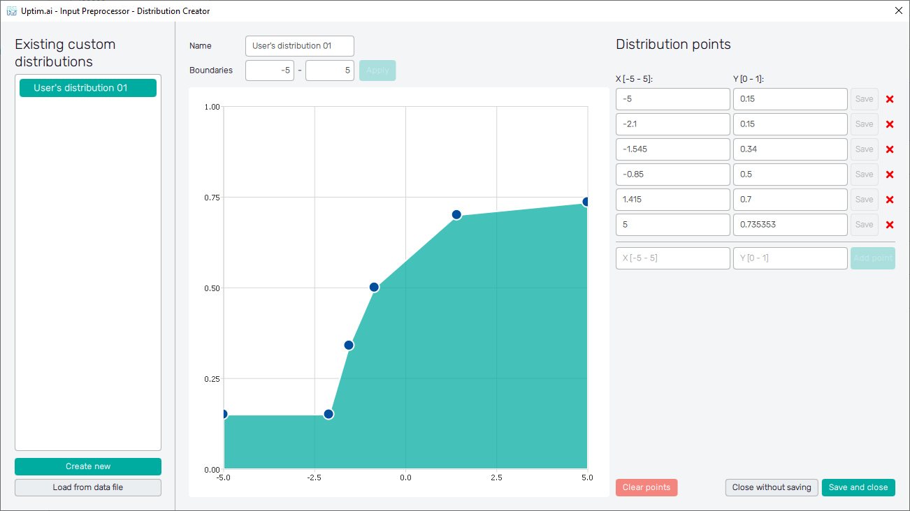
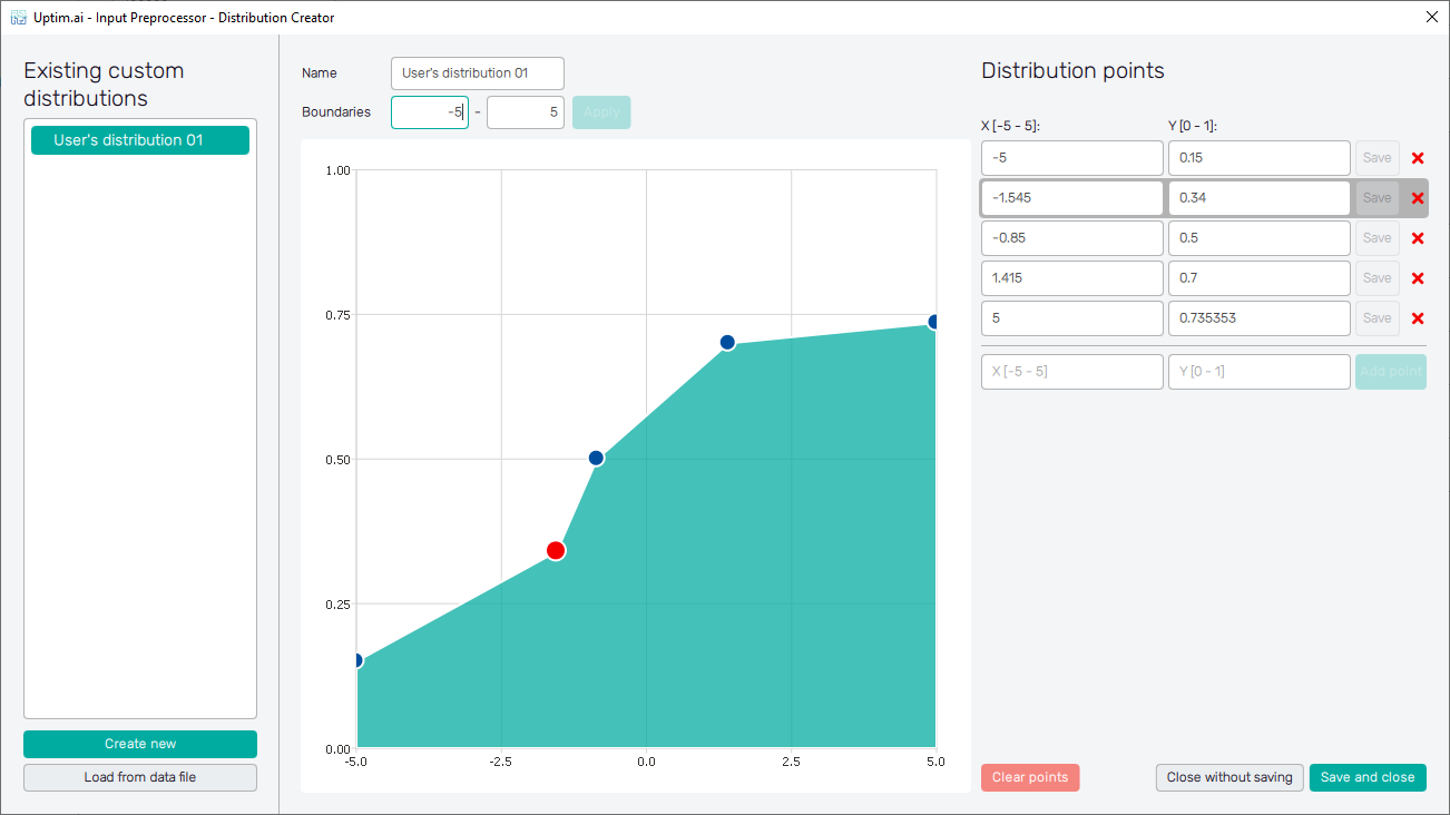
As shown in Figure 12, all created definition points are listed in the list of entries on the right side of the window, one row of the table for each point. Within the limits given by boundaries, positions and weights of definition points can be edited. Confirmation of changes is required and done using the Save button. For better clarification, the edited point is highlighted in the canvas area (vice versa the definition point manipulated in the canvas area gets highlighted in the table). At the bottom of the table of points, there is a possibility to add a new definition point by inserting its exact coordinates into empty entries and confirming with the Add point button. If necessary, for both adding and editing definition points of the distribution, their order in the table changes automatically to keep their position coordinates in ascending order. Similarly, each distribution point can be removed by clicking on the corresponding X button in the table (see Figure 13).
To start with the distribution shape again, one can use the Clear points button underneath the table. Two remaining buttons deal with the closing of the Distribution Creator window. Close without saving button discards the window without any effect on the project. The Save and close button adds the newly created input distribution to the project. Then, the distribution can be found and selected in the list of available input distribution types (see Figure 14).
Files of each user defined distribution shape are stored in a dedicated subfolder inside the
custom_distributions folder, located inside the project. There are two files: info.json
with general information about the distribution name and boundaries, the points.csv contains a
table of the distribution points' coordinates.