Design of Experiment
This is a basic tutorial of Uptimai software prepared to give a first introduction to the suite,
and how to run its different features. To complete this tutorial there will be needed the
Uptimai software and optionally a *.zip file with some complementary files required for the example
problem to be solved. The OTL.zip file can be found inside Uptimai Member Area ->
Downloads -> Tutorial cases.
The OTL.zip file contains the whole project folder with the OTL circuit function,
so the user can start at any step of the given
tutorial. Nevertheless, if the user wants to fulfil the tutorial from the beginning, no additional
files are necessary, and it is possible to finish the tutorial just by following this document.
This tutorial will show you:
- How to start the project
- How to run the Input Preprocessor
- What are the main features of the program and how to use them
- What are the results you can expect
Part 1: Launcher
1.1: Start the program
Open the Uptimai software. You can use the Start menu or desktop shortcut if this option was selected during the installation process, or find the executable inside the installation folder
1.2: Begin the project
Create a New Project. You will have to choose an empty folder where all the project files will be located. The name of the folder will become the name of the project, in this example, we will use the name OTL. You can create the folder directly from the interface.
Once you have created the project, an *.uptim file will appear inside your project folder.
That file is used as a flag so the folder is recognized as an Uptimai project, and contains
the information about already available sets of input files, setups, etc.
The basic rule for the
*.uptim file is the file name has to be the same as the name of the project folder.
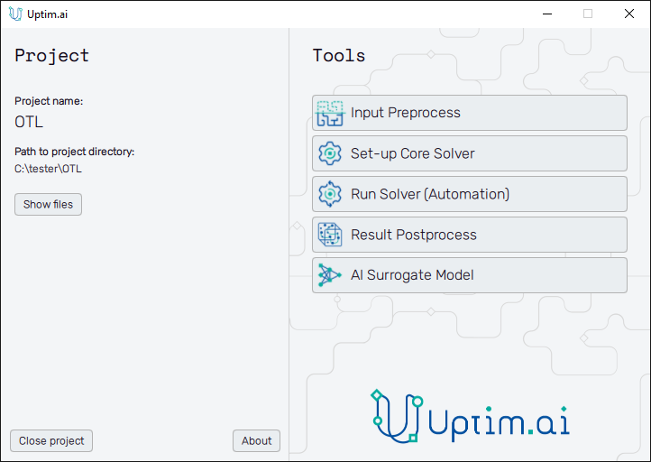
1.3: Proceed to Tools
Now, you have access to all the different features that conform to the Uptimai suite. In this tutorial, we will use them one by one.
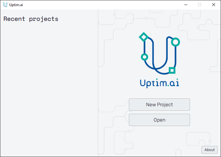
To switch between projects if needed, close the current one with the Close project button at the bottom left of the window and use the Open button of the Launcher (see Figure 1) to run another one.
Part 2: Input Preprocess
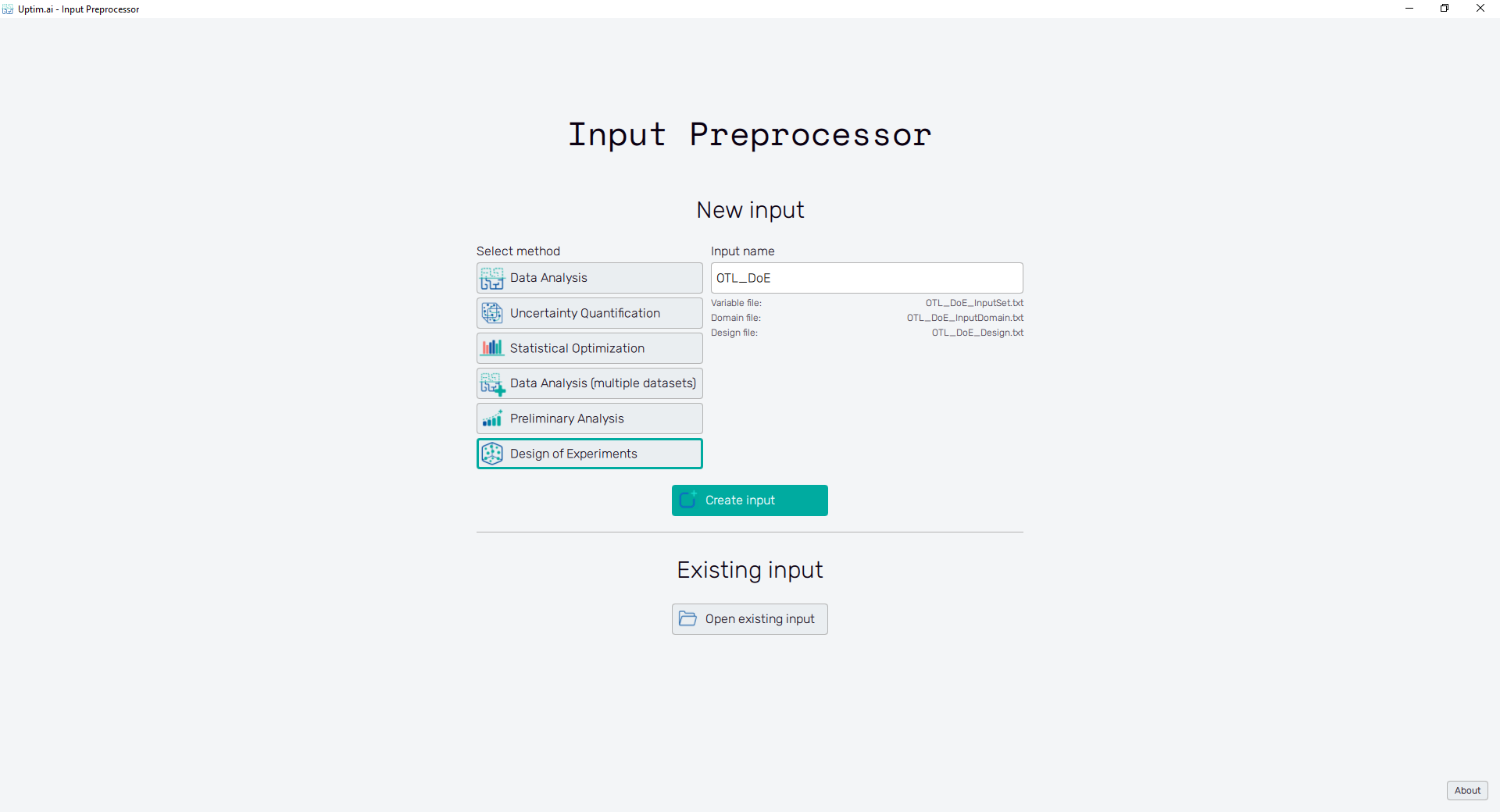
2.1: Open the Input Preprocessor tool
The first step of all projects is always the Input Preprocessor, which can be opened directly from the Launcher. The initial state can be seen in Figure 3. In this tutorial, we will use the Design of Experiment method. It is possible to modify the Input name, but for simplicity, we will maintain the default name suggested by the software. Then, we can click the Create input button to start generating the set of input files.
2.2: Add input variables
In this case, we have 6 input variables, so we will use the Add input variable button at the upper right to generate 6 variable slots.
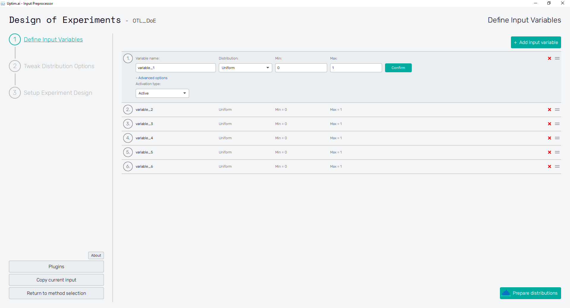
2.3: Define input variables
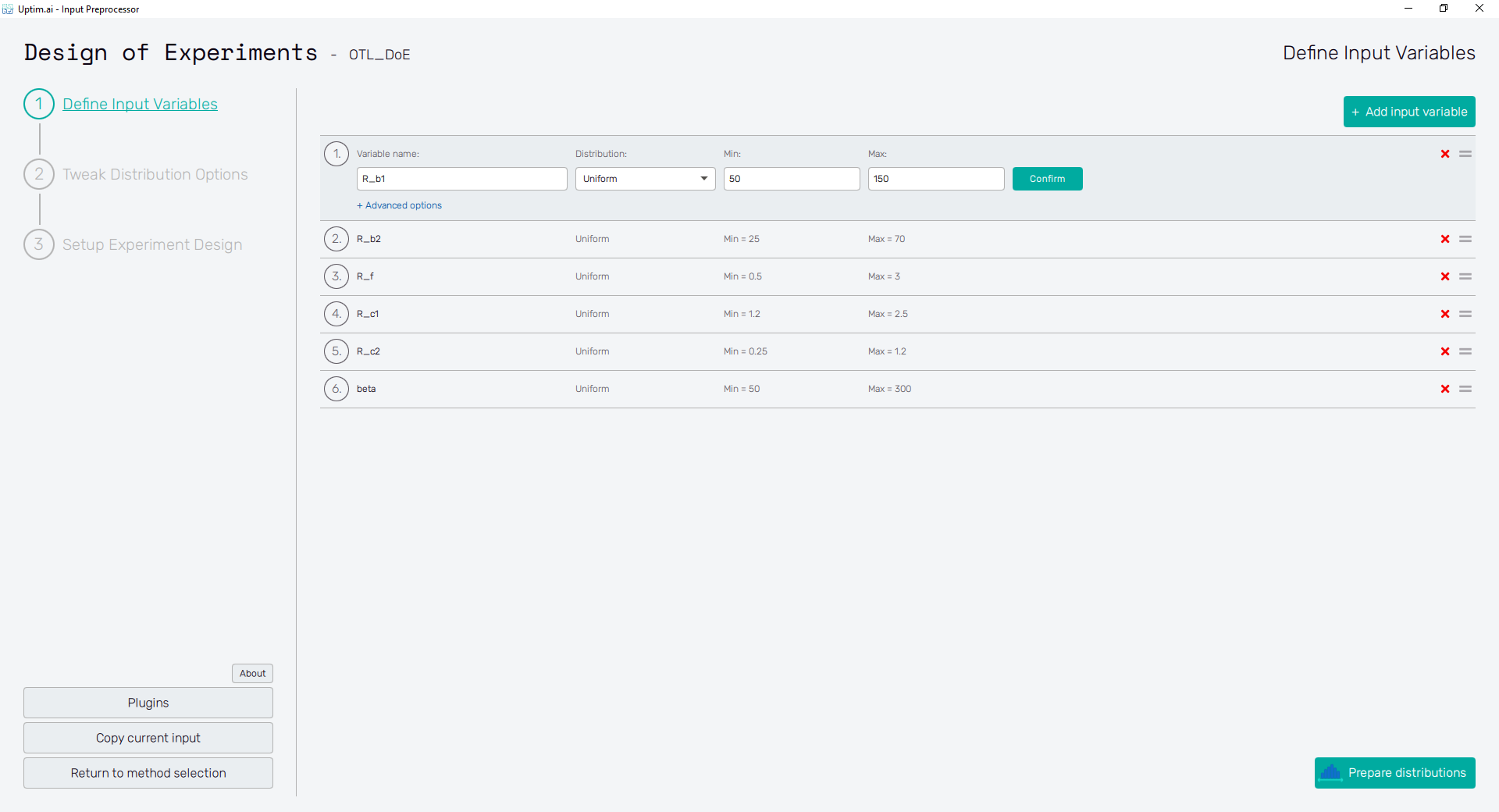
Insert the following distribution to each variable. Remember to press the Confirm button to save the changes after editing each variable. In the end, you should have the same settings as in Figure 5.
Open to view Input Distributions
| Name | Type | Parameter 1 | Parameter 2 |
|---|---|---|---|
| R_b1 | Uniform | 50.0 | 150.0 |
| R_b2 | Uniform | 25.0 | 70.0 |
| R_f | Uniform | 0.5 | 3.0 |
| R_c1 | Uniform | 1.2 | 2.5 |
| R_c2 | Uniform | 0.25 | 1.2 |
| beta | Uniform | 50.0 | 300.0 |
2.4: Prepare distributions
With all input variables defined completely, the program will compute mean values (and boundaries, if necessary) of assigned probability distributions. The Prepare distributions button will then morph into the Tweak distribution options button.
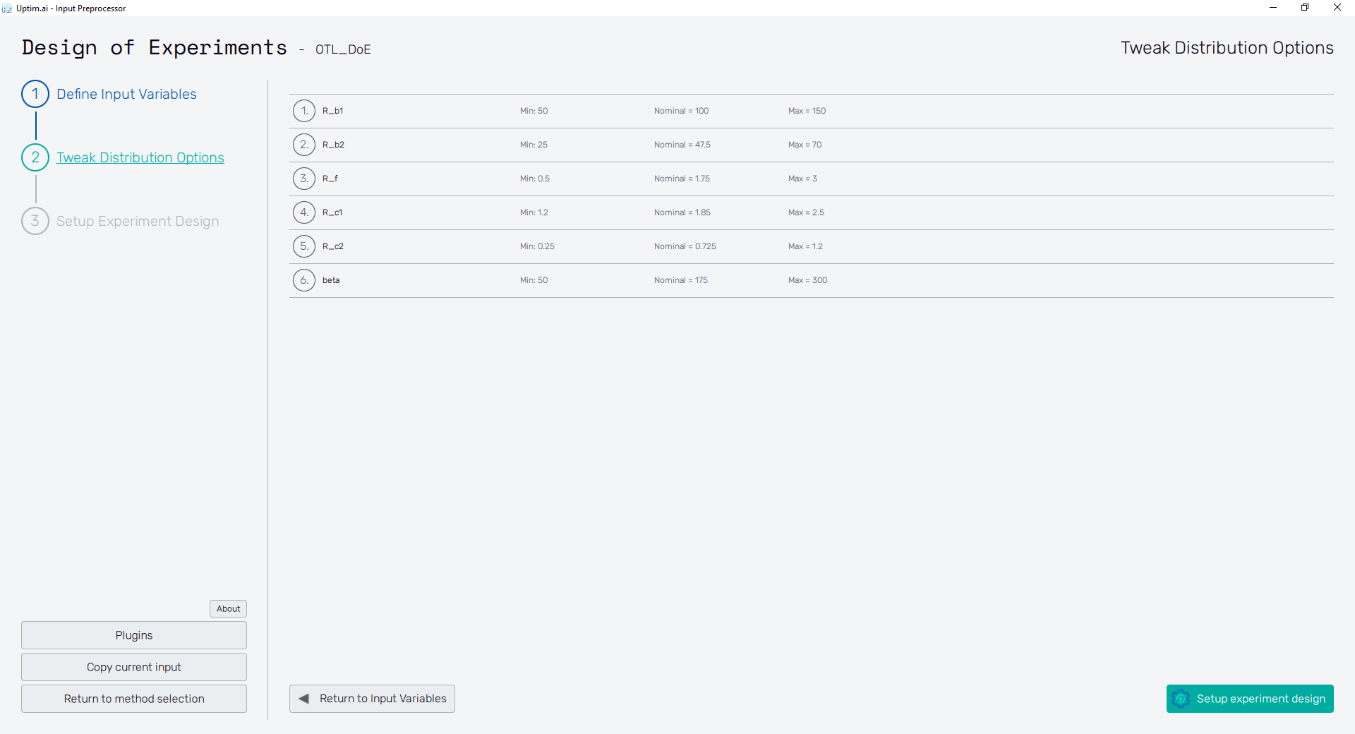
2.5: Tweak Distribution Options
The Tweak distribution options button in the bottom right of the screen or the item of the fishbone navigation bar on the left switches to the Tweak Distribution Options screen. Boundaries of input distributions are adjusted here as well as the position of the nominal sample.
By default, the nominal sample position is set to be the mean value of each input distribution. It is recommended to keep in not further from this point than 10% of the input distribution range. For our current case, there is no need for adjustments of the boundaries or nominal values. All input files are created and saved upon the Generate data button clicking. Then, this button's label turns to Setup Experiment design and the following section becomes accessible.
Design of Experiment
Since we are covering only the Input Preprocessor tool in this tutorial, this is a separate section of Part 2 of the tutorial focusing on the implemented Design of Experiment techniques and the work with corresponding features of the program.
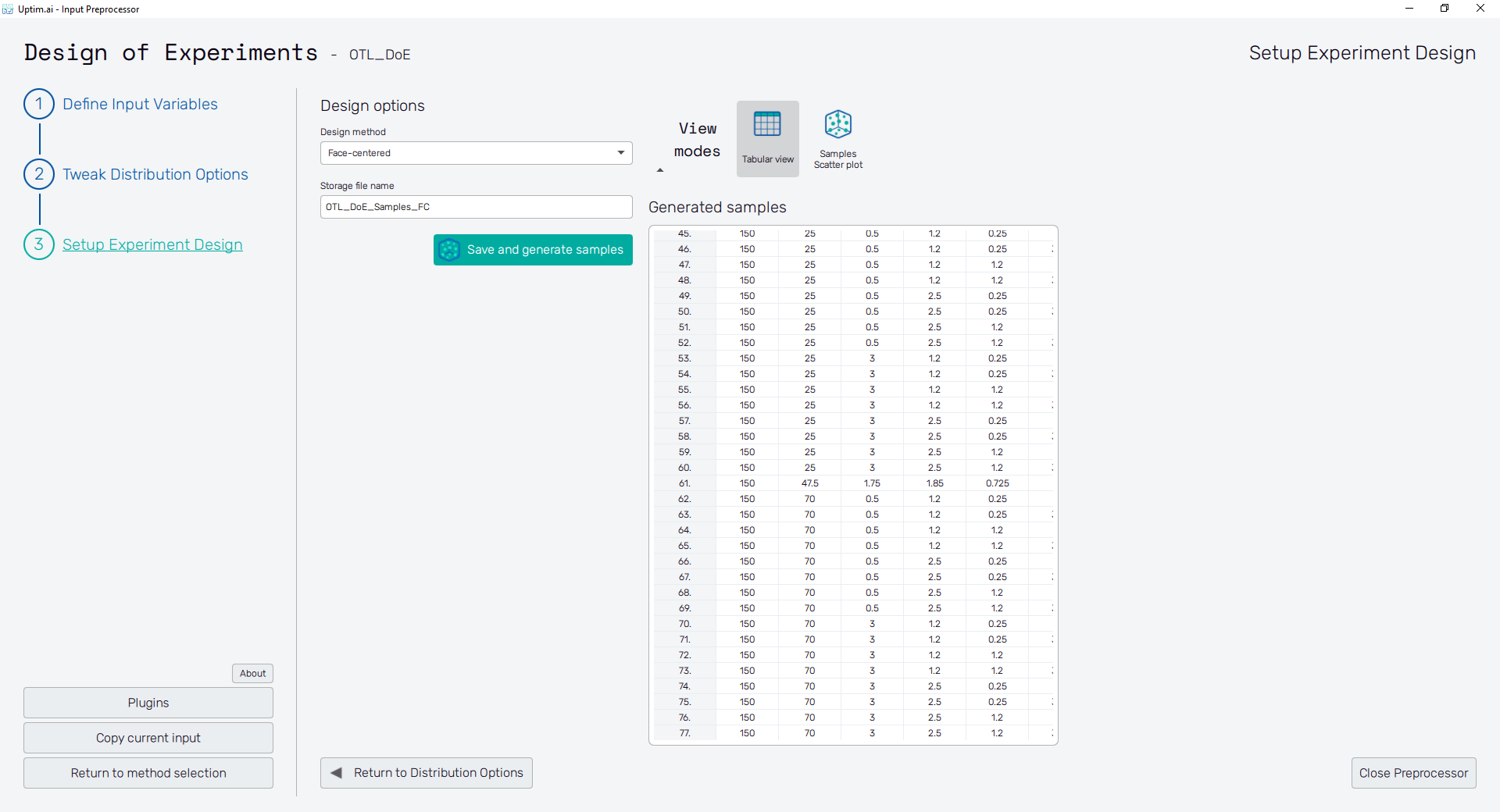
2.6: Setup Experiment design
In the Design options menu find the Design method selector. Let's assume we are in the stage of the project where our main goal is to perform the Sensitivity Analysis. For this purpose, the Face-centered design that covers domain edges is the right choice. Select this option from the menu.
The number of samples generated is given by the design method itself and cannot be modified in this
particular case. Change the Storage file name of the *.txt where the table with coordinates of
generated samples will be stored, e.g. to OTL_DoE_Samples_FC. Now you can use the Save and
generate samples button to let the method work.
2.7: Check generated samples in table
Samples are shown immediately after they are generated. The default screen is the Tabular view where you can see all samples in the exactly same order as they are stored in the file.
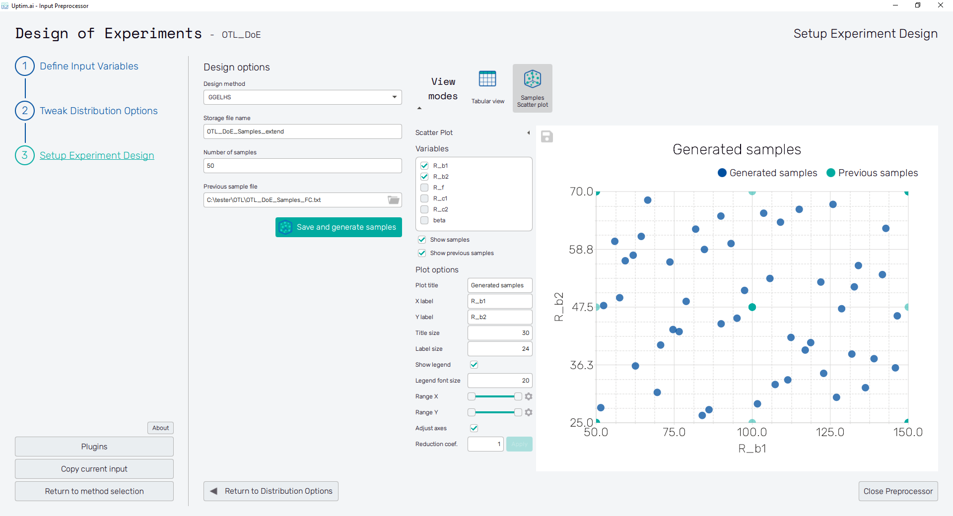
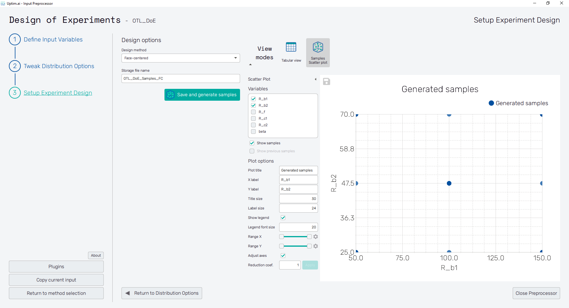
2.8: Review generated samples in scatter plot
Switching to the Samples Scatter plot feature you can see the actual distribution of samples in the domain. Play with checkboxes of the list of Variables on the left. You can select up to two input variables to be shown in the plot. Adjust Plot options and save the figure using the 💾 icon in the top left corner of the plot.
Add samples to the design
Since the next step of the project would be the computation of the model, let's generate a set of additional samples to cover also the blank spaces of the domain. We want to enhance the existing set of samples, thus, we will use the GGELHS method to complement it with up to new samples.
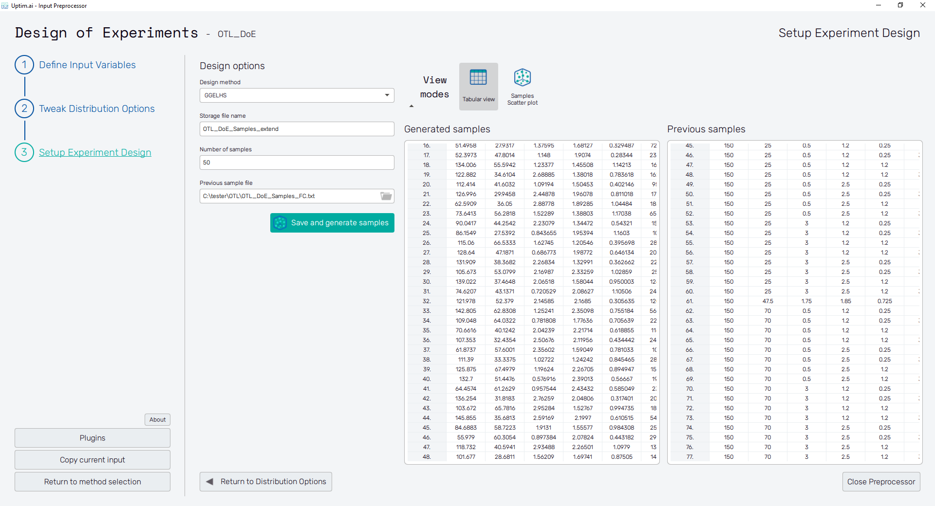
2.9: Generate additional samples
Find and select the GGELHS in the list of Design methods in the Design options menu. There will be the Storage file name entry we saw already in step 2.6. Right underneath you need to define the Number of samples to be generated as compliant to the Latin Hypercube. Here we will put the number , but it is possible that fewer samples will be actually generated since the GGELHS method tries to consider already existing samples.
2.10: Review generated samples in scatter plot
Check the Samples Scatter plot feature to see both sets of samples side by side. All you need to do is to check the Show previous samples item of the Scatter plot control panel on the left. Again, you can select up to two input variables to be shown in the plot. Adjust Plot options and save the figure using the 💾 icon in the top left corner of the plot.