Design of Experiments
The Uptimai Design of Experiments method builds sampling schemes commonly used in operational research. It also allows the enhancement of the existing matrix of data points with new members to optimally fill the design space when increasing the precision of the data approximation. The method can be used separately or as an initial step of the Data Analyzer method.
How to use the interface
The general appearance of the program window, especially its left section, is described in detail in the Input preparation link. Here the main focus is on the other part which is to a certain point individual for each of the supported methods. The initial of the GUI window when preparing inputs for the Design of Experiments is shown in Figure 1, as the user starts from scratch and needs to Define Input Variables.
Define Input Variables
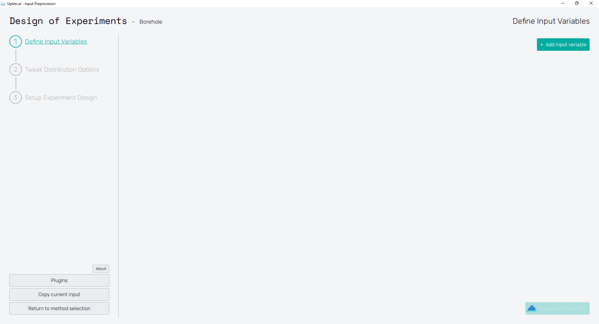
In the beginning, the user creates a new variable (parameter) of the input domain with the Add input variable button. Each added variable appears at the bottom of the list of already existing variables.
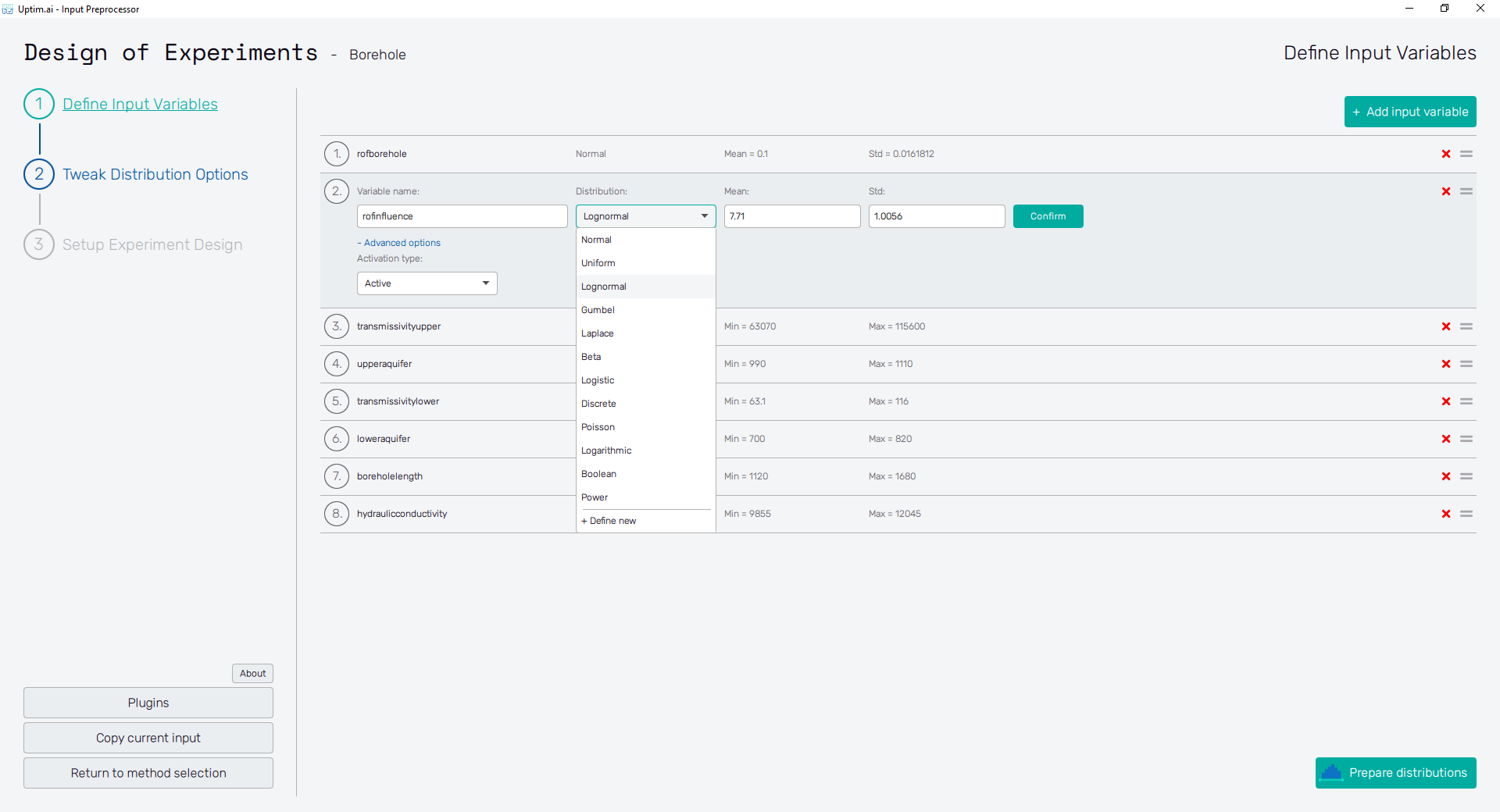
Adding an input variable enhances the input domain space with one dimension. There has to be at least one for the model to be created. Figure 2 describes the situation with multiple input variables already created (see this link for more info about the borehole problem). One of the displayed variables is about to be edited. The input variable can be set using the following controls:
- Variable name : Label of the input parameter, which is being used throughout the whole process up to the postprocessing. The variable name cannot contain empty spaces, these are automatically replaced with underscores.
- Distribution : Selection box where the user sets the shape of the probabilistic function for the input variable. According to the distribution type selected, additional entries with shape parameters appear. A detailed description of featured probability distribution types can be found in the section Input distribution types.
- Confirm : Any changes need to be confirmed with this button to take effect.
- "X" : Each input variable can be deleted when clicking this icon.
- "=" : Allows input variable dragging to change the ordering of inputs in the projects.
Adding one or more input variables activates the Prepare distributions button. This one invokes the preparation of randomly distributed samples according to the settings. In case there are invalid entries in the input variable definition, the user is informed and not allowed to continue to the next step until everything is by the book. Then, the button itself turns into Tweak distribution options, sending the user to this next step. Also, the Tweak Distribution Options item is activated in the fishbone navigation bar on the left.
Tweak Distribution Options
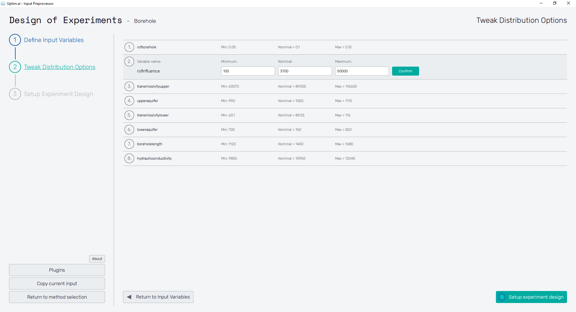
At this point, the user adjusts the boundaries of the input domain and the so-called nominal sample. Boundaries are recommended to be adjusted especially for distribution shapes where the user defines parameters like mean value and standard deviation. In these cases, the edges of the domain depend on the randomization of samples within the input variable. Thus, modification is usually required to set the exact range for such inputs. For certain types of distribution shapes like uniform or discrete, edges of the domain are exactly given by the distribution shape definition and cannot be changed after.
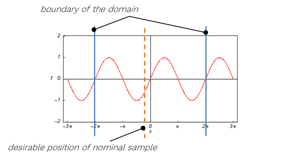
The nominal point is a sample acting as a baseline for the created surrogate model and analysis. In the model, the results of all data samples are compared with the result value of the nominal sample. This process allows handling the effects of input parameters and their interactions separately as increments to the nominal value. It must be within the range of each input variable and not be equal to its boundaries. Although not strictly necessary, it is recommended to place the nominal sample into the statistical centre of the domain. Then, the process of the surrogate model creation is most efficient and precise. The nominal sample's default position is suggested as the mean of the probability distribution of each input variable. When changing its position, (shown in Figure 3) it is advised not to shift it by more than 10% of the range of each input. As in the case of input variable distribution definition, all changes must be saved using the Confirm button.
For the sampling of variables leading to periodic or symmetrical functions (typically, but not exclusively, angles of any kind), extra caution is required. It is highly recommended not to set their nominal value exactly to the centre of symmetry of the corresponding input distribution! A typical example can be the angular position of a crankshaft, wave phase, etc.
Clicking the Generate data button at the bottom right invokes the saving
of .txt files with randomly distributed samples according to the settings and input domain info.
Then, the button itself turns into the Setup Experiment Design,
sending the user to this next step. Also, the Setup Experiment Design item is activated
in the fishbone navigation bar on the left. For fundamental changes in any of the input distributions
can the user go back to the previous step with the Return to Input Variables button.
Setup Experiment Design
Here the user creates the matrix of data samples' coordinates. To the right from the fishbone navigation bar, there is the Design option section where one can choose the sampling method. Currently, the following methods commonly used in the response surface methodology are featured:
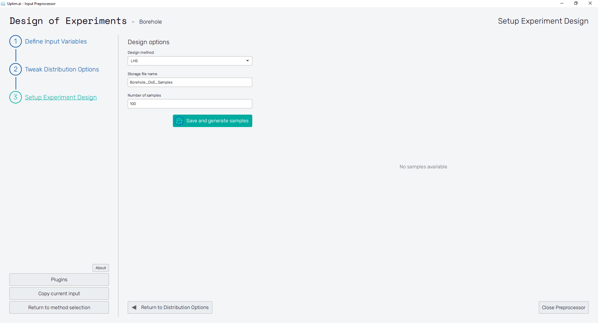
- LHS : Latin hypercube sampling is used to create randomly distributed samples across the domain, which is then covered optimally in all dimensions. Each input variable distribution respects the distribution shape selected in the Define Input Variables section. The number of samples needs to be set by the user in the Number of samples entry field.
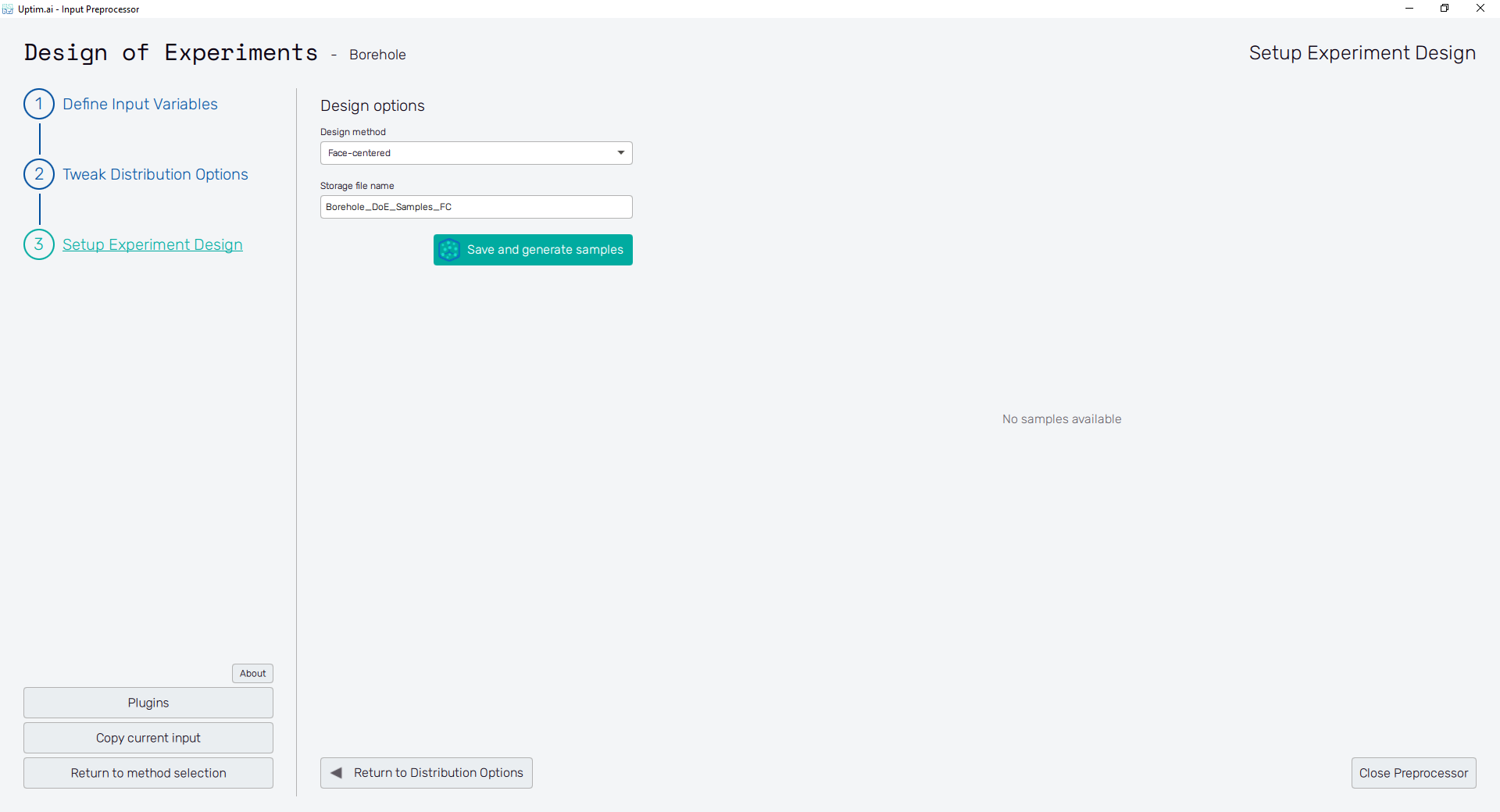
- Face-centered : The type of central composite design (CCD) method, where all samples (besides the central point) are located on the edges of the domain. Offers good quality of domain coverage, however, might not give the best performance for models containing quadratic shapes. The number of samples is fixed and depends on the number of input variables.
- Box-Behnken : Very efficient design scheme for cases with a low number of parameters. Does not contain points in corners of the domain, thus, a model based on Box-Behnken can be insufficient in describing the effects of combined extremities of input parameters. The number of samples is fixed and depends on the number of input variables.
- BGELHS : Basic General Extension algorithm of LHS. When adding new samples to the domain, this method reuses as many existing samples as possible in the new set, however, some previous samples might get lost anyway. BGELHS can be significantly time-consuming for larger domains with a higher number of input variables and a higher total number of required samples.
- GGELHS : General Extension Algorithm of LHS Based on Greedy Algorithm. Allows to add samples to the domain. Not as effective in sense of the number of samples kept from the previous run as BGELHS, but works much faster.
For further information about methods and algorithms used for domain space sampling check the links here and here.
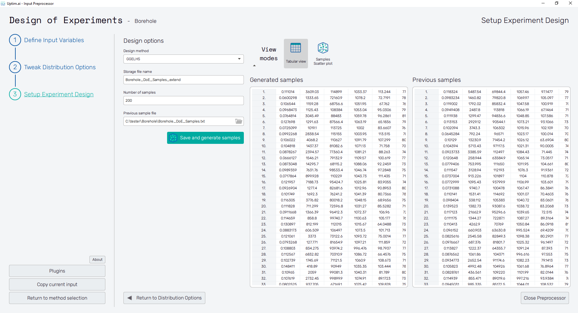
Clicking the Save and generate samples button generates samples according to the selected method and shows the coordinates of created points in the table on the right as Generated samples. If needed, the process can be stopped using the Cancel button, which appears while the samples are being generated.
Created samples are stored in the *.txt file
named as set in the Storage file name entry field. This file can be found in the project folder
and it is loaded automatically if it already exists as a result of the previous work.
Two more buttons are located under the table. Return to Distribution Options brings users back
to the previous step Tweak Distribution Options where they can fix boundaries or the
position of the nominal sample. The other button will Close Preprocessor.
Also, additional features are accessible after samples are generated. Their icons labelled Tabular view and Samples Scatter plot will appear on the top of the window
Tabular View
In this feature one can review the generated samples in the form of a spreadsheet. Since the feature only displays the data as they are stored in the file, it does not allow to sort or modify these.
For BGELHS and GGELHS designs methods, there is one more table present in the screen. The table with Previous samples shows the content of the Previous sample file.
Samples Scatter Plot
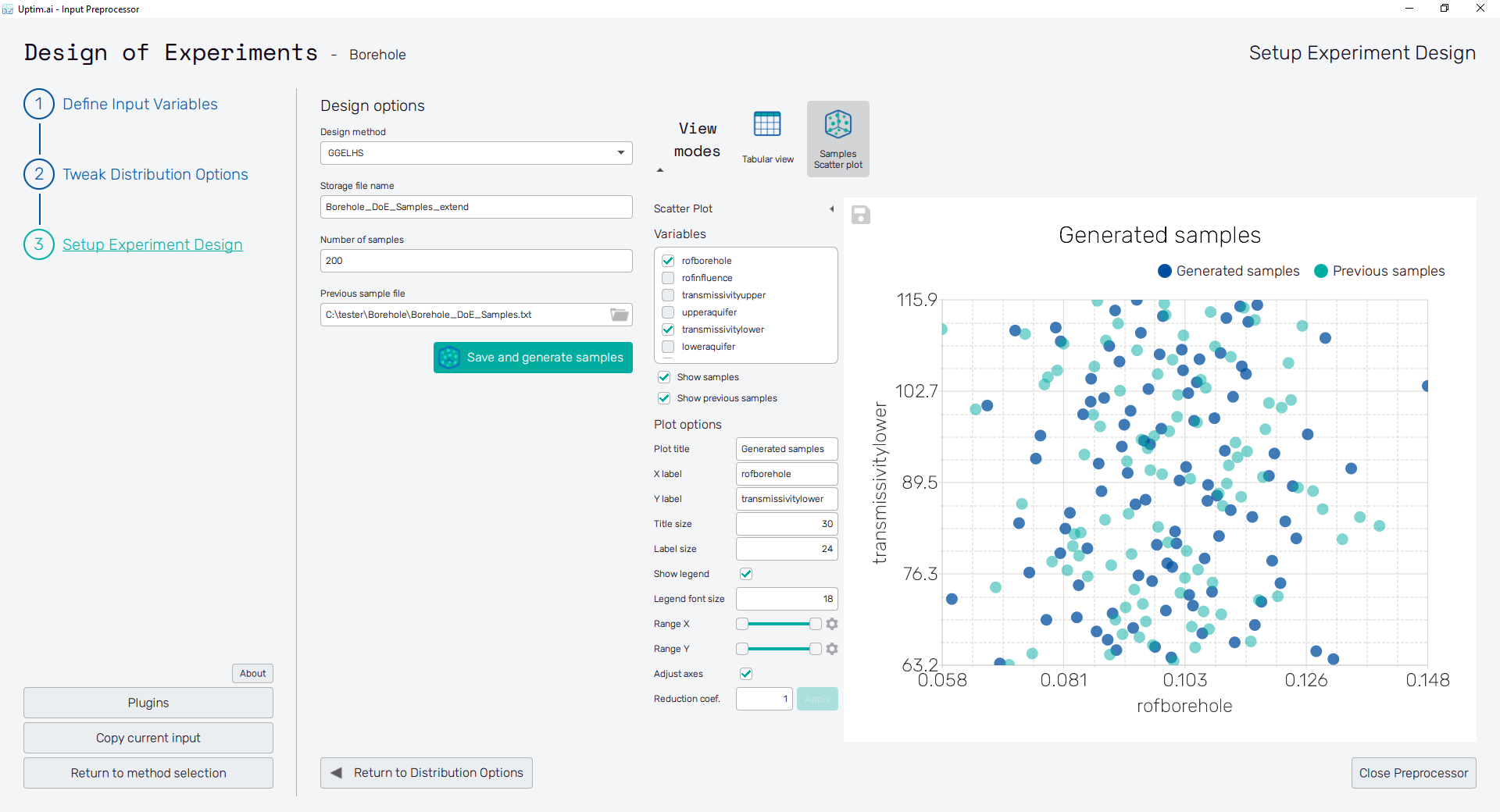
To export the plot as a .png or .jpg file, the save-file dialogue can be induced
by clicking the 💾 icon on the top left of the plot.
It is possible to adjust the appearance of the plot using controls from
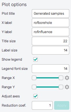
the Plot options section of the panel on the left:
-
Plot title : Displayed above the plot, Generated samples by default.
-
X label : Label of the X axis, name of the only or the first selected input variable by default.
-
Y label : Label of the Y axis, name of the only or the second selected input variable.
-
Title size : Size of the title font.
-
Label size : Size of the label font.
-
Show legend : Switching on/off the legend of the plot/the colorbar scale.
-
Legend font size : Size of the legend font.
-
Range X : Double-sided slider allowing to show a slice of the data in detail. Dragging one of the slider's points limits the depicted range of input variable values, one can move with the section along the X-axis by dragging the green bar of the slider (both edge points are highlighted).
-
Range Y : Double-sided slider allowing to show a slice of the data in detail. Dragging one of the slider's points limits the depicted range of input variable values, one can move with the section along the X-axis by dragging the green bar of the slider (both edge points are highlighted).
All ranges in the plot can be also precisely using the ⚙ icon on the right of each slider. This opens a sub-dialogue with entry fields for writing exact values of range limits. These need to be confirmed with the Set button. Setting values outside the domain's boundaries will reset range limits to the default state.
-
Adjust axes : Toggle if the axis and/or colorbar limits of the plot should be only the range adjusted with the slider above (on) or the full range of the input distribution (off).
-
Reduction coefficient : Variable that reduces the total number of samples that are plotted for an easier interpretation of results. If set to , the whole set of loaded samples specified will be depicted.