Data Analysis - Multiple Datasets
The Uptimai Data Analysis - Multiple Datasets builds multiple surrogate mathematical models over one domain at once. In the end, all models can be carefully examined as described for regular Data Analysis result files, using all the available features. Moreover, it is possible to study relations between multiple outputs related to the modelled problem. Also, it detects anomalies in the data, locates these, and helps to recognize the type of error that may be present in the set source measurements.
This is a basic tutorial of Uptimai software prepared to give a first introduction to the suite,
and how to run its different features. To complete this tutorial there will be needed the
Uptimai software and a *.zip file with some complementary files required for the example
problem to be solved. The AnomalyDetection.zip file can be found inside Uptimai Member Area ->
Download -> Tutorial cases.
The AnomalyDetection.zip file contains the whole project folder, so the user can start at any step of the given
tutorial. The example project represents a datalog of simulated rocket launch telemetry.
Nevertheless, if the user wants to fulfil the tutorial from the beginning, only the
set of *.txt files with input matrices will be necessary, as all the other files will be generated
during the process. These can be found in the input_matrices_anomaly subfolder of the prepared
example project.
This tutorial will show you:
- How to start the project
- How to run each program of the package
- What are the main features of each program and how to use them
- What are the results you can expect
- How to export and store output data
- How to generate the report
Part 1: Launcher
1.1: Start the program
Open the Uptimai software. You can use the Start menu or desktop shortcut if this option was selected during the installation process, or find the executable inside the installation folder
1.2: Begin the project
Create a New Project. You will have to choose an empty folder where all the project files will be located. The name of the folder will become the name of the project, in this example, we will use the name AD (for Anomaly Detection). You can create the folder directly from the interface.
Once you have created the project, an *.uptim file will appear inside your project folder.
That file is used as a flag so the folder is recognized as an Uptimai project, and contains
the information about already available sets of input files, setups, etc.
The basic rule for the
*.uptim file is the file name has to be the same as the name of the project folder.
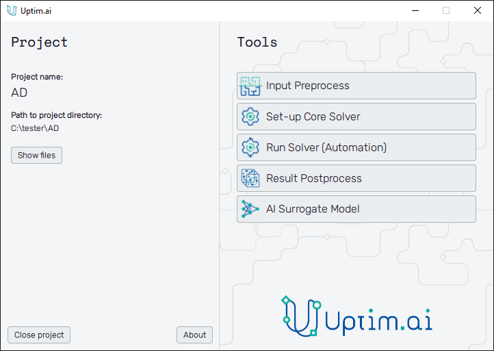
1.3: Proceed to Tools
Now, you have access to all the different features that conform to the Uptimai suite. In this tutorial, we will use them one by one.
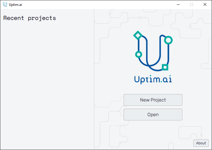
To switch between projects if needed, close the current one with the Close project button at the bottom left of the window and use the Open button of the Launcher (see Figure 1) to run another one.
Part 2: Input Preprocess
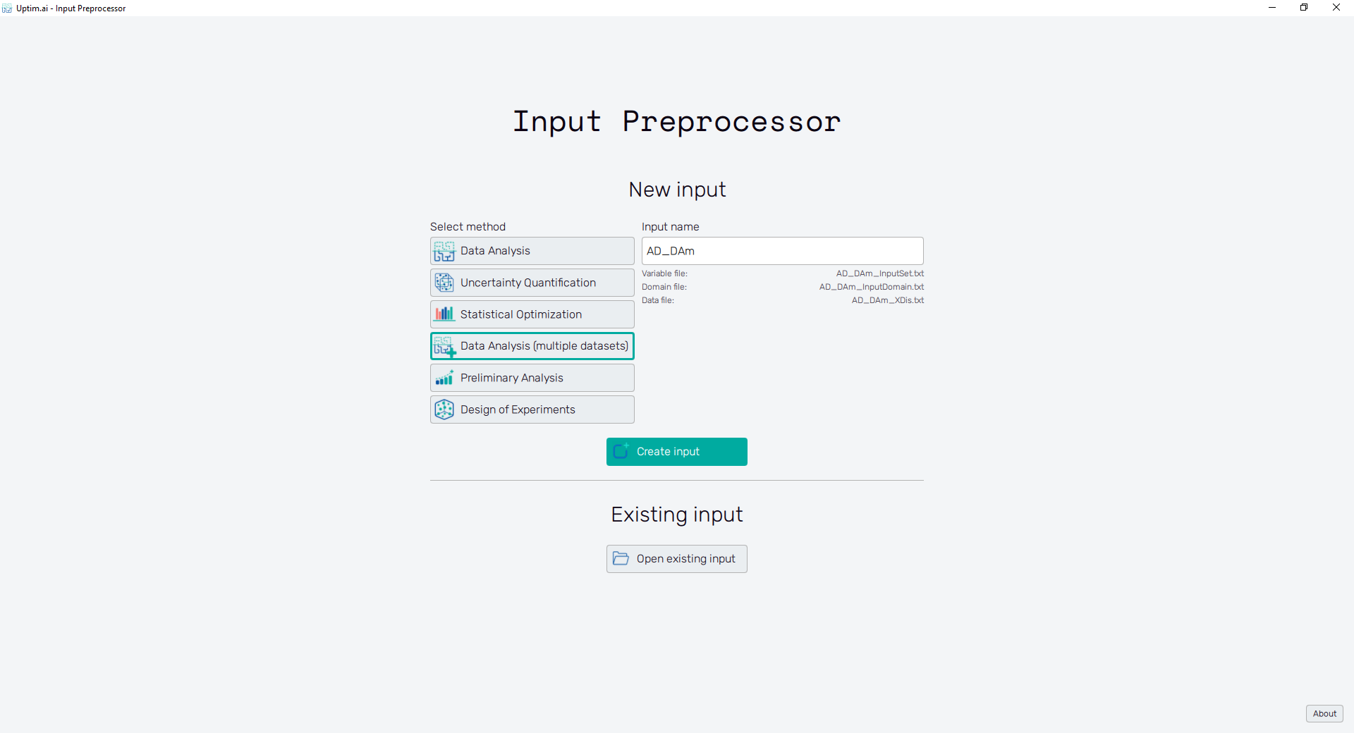
2.1: Open the Input Preprocessor tool
The first step of all projects is always the Input Preprocessor, which can be opened directly from the Launcher. The initial state can be seen in Figure 3. In this tutorial, we will use the Data Analysis (multiple datasets) method. It is possible to modify the Input name, but for simplicity, we will maintain the default name suggested by the software. Then, we can click the Create input button to start generating the set of input files.
2.2: Select training data
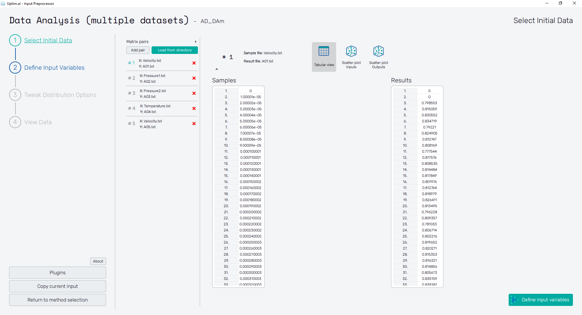
When starting with the new set of inputs for the Data Analysis (multiple datasets) method, the process begins with the Select Initial Data screen. In the current project, we will compare five different outputs, thus, we have to load five related pairs of measured data. Use the Add pair button at the top of the screen to invoke the file-selecting dialogue. Here select pairs of Sample matrix files and Result matrix files to get the final list as shown in Figure 4 (all files can be found in the input_matrices_anomaly folder of the downloaded project example).
Open to view list of matrix pairs
| Pair | Sample matrix file | Result matrix file |
|---|---|---|
| # 1 | Velocity.txt | A01.txt |
| # 2 | Pressure1.txt | A02.txt |
| # 3 | Pressure2.txt | A03.txt |
| # 4 | Temperature.txt | A04.txt |
| # 5 | Vibration.txt | A05.txt |
Immediately after creating each pair of source data files, you should be able to see their content in the form of two tables. Do not be alarmed that the domain (list of variables and ranges of their inputs) gets reset after each pair of matrices is defined. Note the table of Samples has only one column stating there will be only one input variable studied.
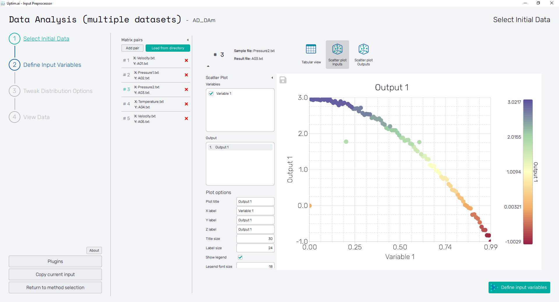
2.3: Scatter plots of Inputs
You can visualize how loaded samples are distributed in the domain with the Scatter plot Inputs feature. See if the input domain is covered evenly: seek for outliers and isolated clusters of samples.
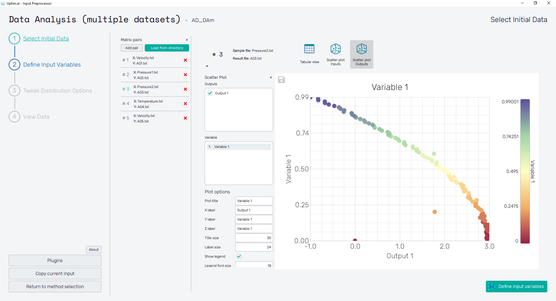
2.4: Scatter plots of Results
A similar visualization can be done vice versa with outputs on the axes of the plot. Just switch to the Scatter plot Outputs to see. Now, the selected Variable defines the color of each depicted sample.
2.5: Define Input Variables
Using the Define Input Variables button in the bottom right of the screen or the item of the fishbone
navigation bar on the left switch to the Define Input Variables screen. Here the situation is pretty
easy since we have only one variable we are working with. This is strictly given by the number of
columns in the file with training samples loaded in step 2.1. Just make sure you set the
Distribution type
to Uniform ranging from to . Also, the Variable name can be changed
to series_1, because we know the variable has a character of a time series measured during a spacecraft
launch. Do not forget to Confirm all changes with the button.
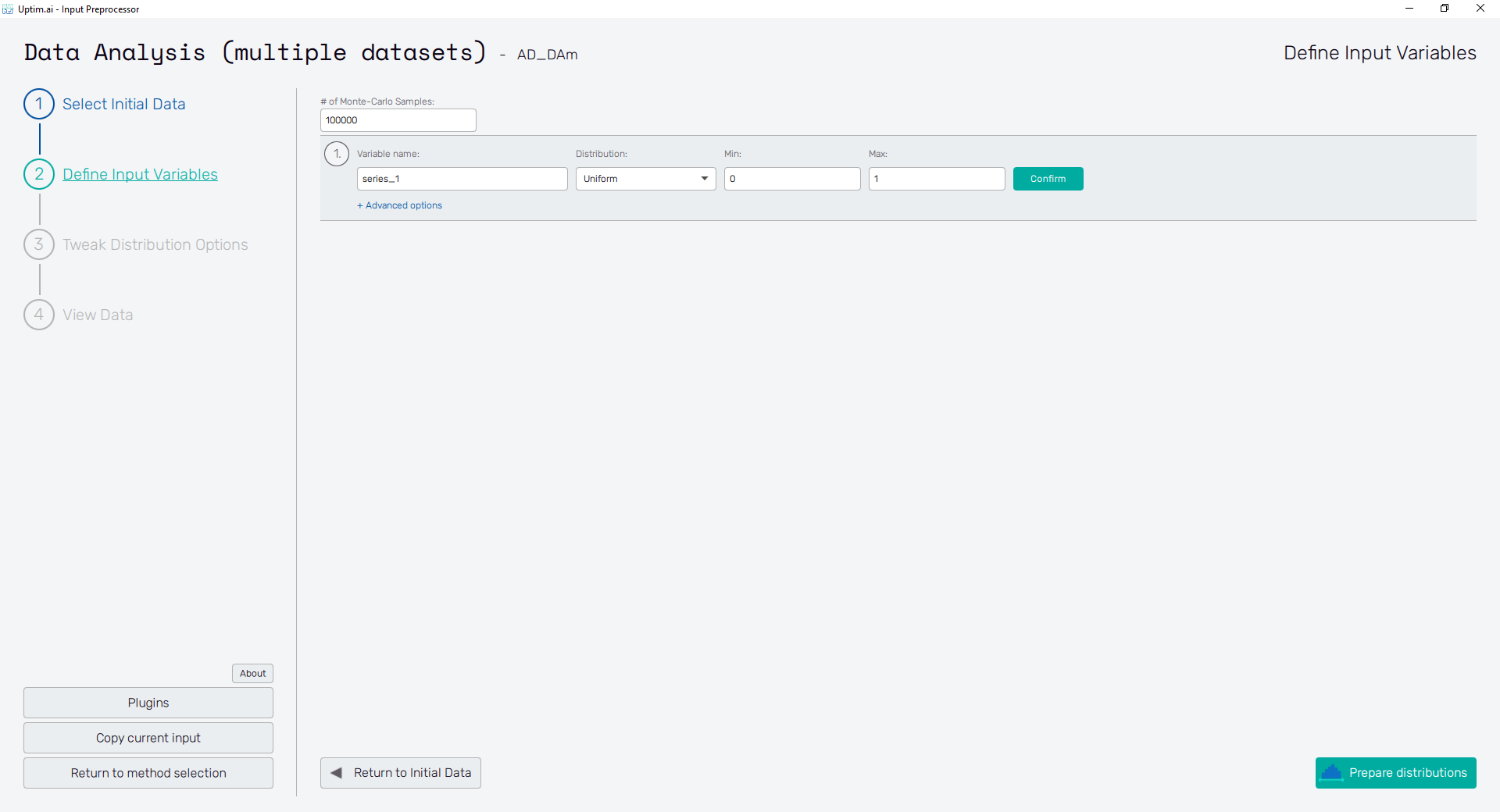
2.6: Prepare distributions
With all input variables defined completely, pre-generate random distributions of samples that will be later used for statistical analysis and visualizations. You can set the number of generated samples in the # of Monte-Carlo Samples entry at the top of the screen.
The Prepare distributions button will generate all distributions according to the setting and then morph into the Tweak distribution options button.
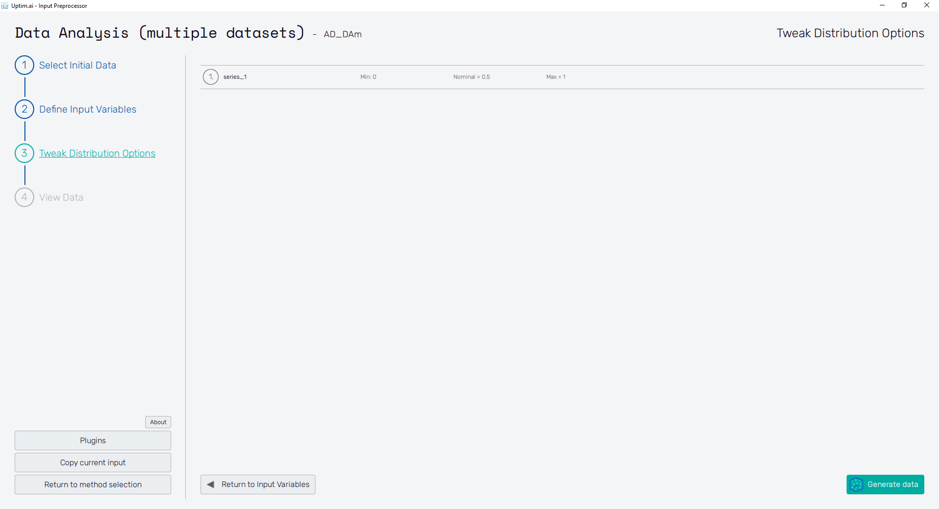
2.7: Tweak Distribution Options
The Tweak distribution options button in the bottom right of the screen or the item of the fishbone navigation bar on the left switches to the Tweak Distribution Options screen. Boundaries of input distributions are adjusted here as well as the position of the nominal sample. There is nothing to be changed at the moment.
By default, the nominal sample position is set to be the mean value of each input distribution. It is recommended to keep in not further from this point than 10% of the input distribution range. All input files are created and saved upon the Generate data button clicking. Then, this button's label turns to View data histogram and the following section becomes accessible.
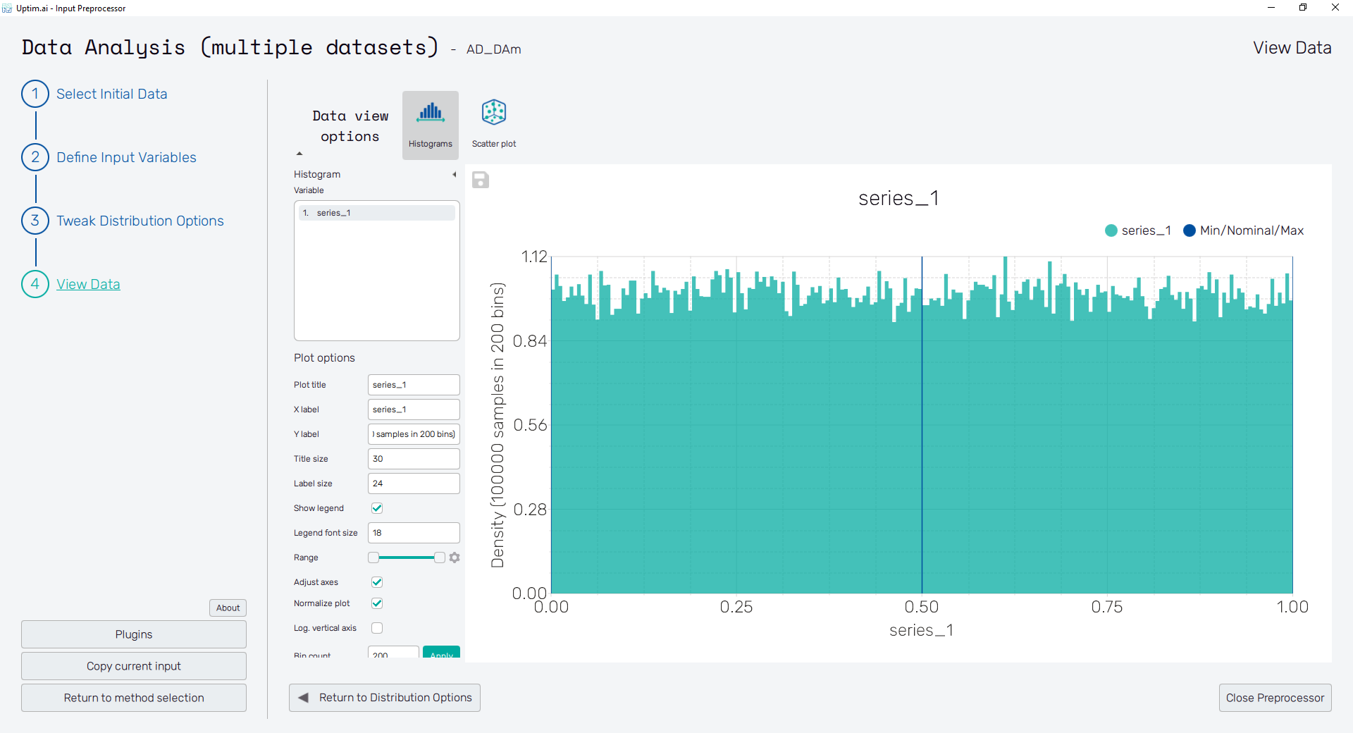
2.8: View Data
Clicking the View Data button in the bottom right of the screen or the item of the fishbone navigation bar on the left shows the View Data screen. Check the presented histogram of the Variable showing the generated probability distributions. You can style the plot using the Plot options section and save it using the 💾 icon located in the top left corner of the plot. Clicking points of interest in the plot shows the pop-up with details. Close Preprocessor button ends the current program.
Part 3: Set up the Core Solver
3.1: Start the setup GUI
Once the inputs have been generated, it is time to prepare all the settings for the solver. We can do that using the Core Solver Setup, which once opened from the Uptimai main interface has the appearance as shown in Figure 10.
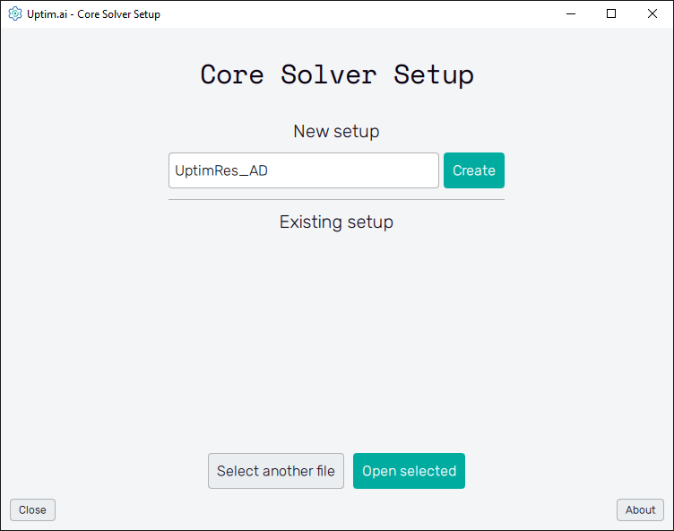
3.2: Create new setup
Once the program is opened, the first thing we need to do is to create a new setup file. We can change the name of the file to UptimRes_AD just to recognize it easily later, and then just click on the Create button.
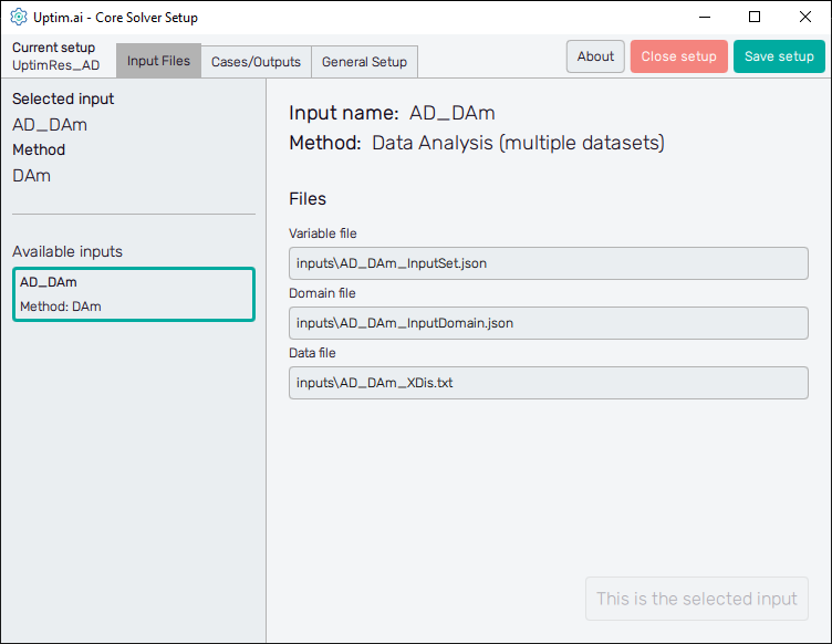
3.3: Select the set of inputs
Then, we will see that the Core Solver Setup has three
main tabs. The first one is to select the input files that will be used in this run.
In our case, we want to use the set of inputs prepared for the
Data Analysis (multiple datasets) method.
3.4: Set up the case
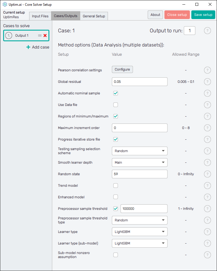
The second tab, which is Cases / Outputs, details all the settings that are used for tuning the core solver to the needs of our problem. Thus, there is a setup specific to the Data Analysis (multiple datasets) method we are working with. Also, there is information about which outputs we would like to study. Output 1 is present at the start, and we will keep it because each of our input matrices contains only one column of values.
Pay special attention to the Pearson correlation settings accessible via the Configure button. It is an important setup for the search for correlated anomalies. Since we do have only one input variable in our problem, there is no need to set the reference input variable. However, we want to discretize its range into bins and set the constant threshold rule for anomaly identification with the limit value of .
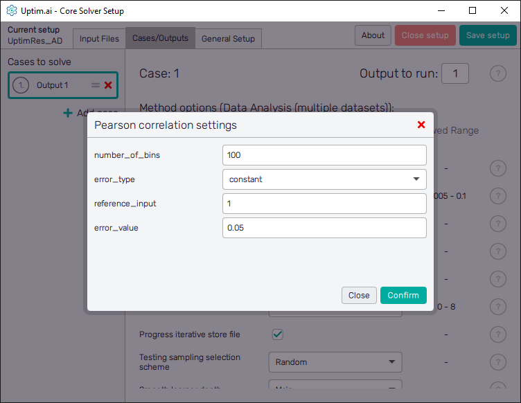
Be sure you have the same setup as shown in Figure 13. Note the LightGBM type of learner is used for both model and sub-models. Be sure you will select these from the drop-down menu. This method is well suited for large datasets such as the one we have here consisting of samples.
3.5: General setup
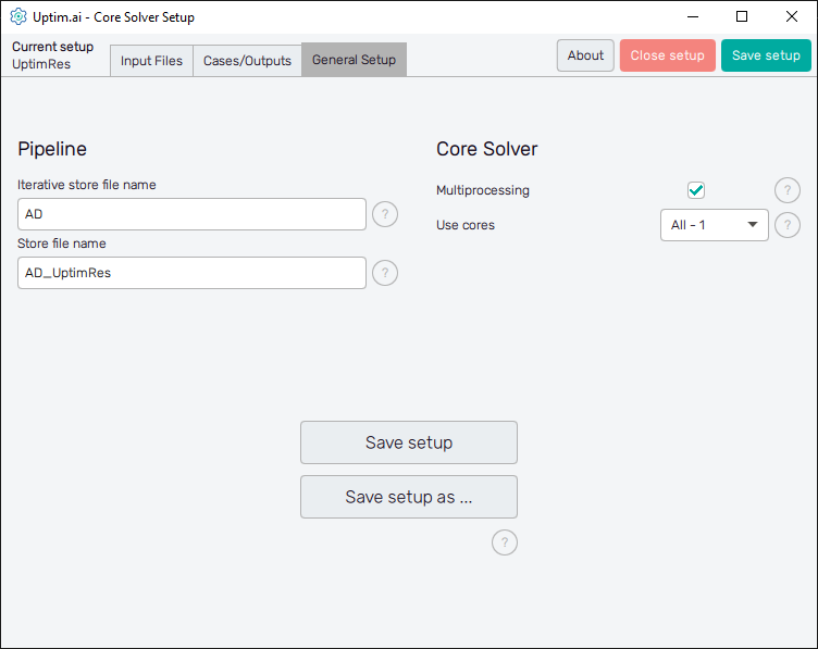
Finally, in the third tab, there is information regarding naming and other solver aspects. In
this case, we don’t need to modify anything, and we can directly save the setup. When we do that,
an UptimRes_AD.json file will be generated in the project folder containing all the information
that we saved. That file will be used by the solver itself.
Part 4: Run Solver (Automation)
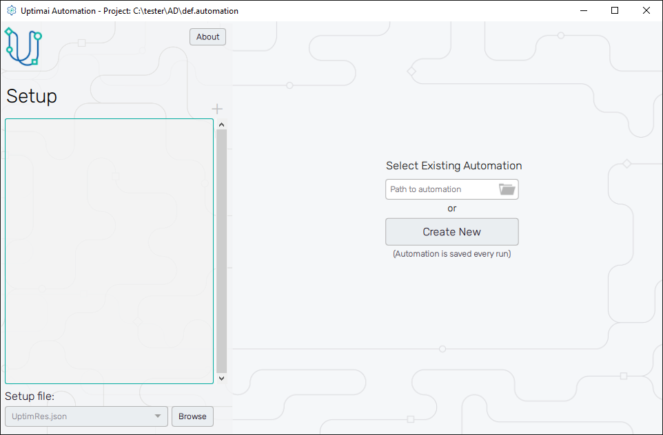
4.1: Create new automation configuration
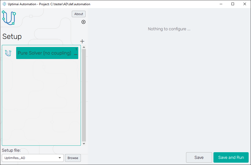
Now it is time to open the Run Solver (Automation) from the Uptimai main interface. We will create a new automation file using the New automation section of the screen. Here, choosing any name and clicking the Create button stores the newly created file in the project folder. In case you want to load a previously created session, select one item from the list of the Existing automation section and confirm with the Open selected button. Eventually, you can search for any automation session under the Select another file button.
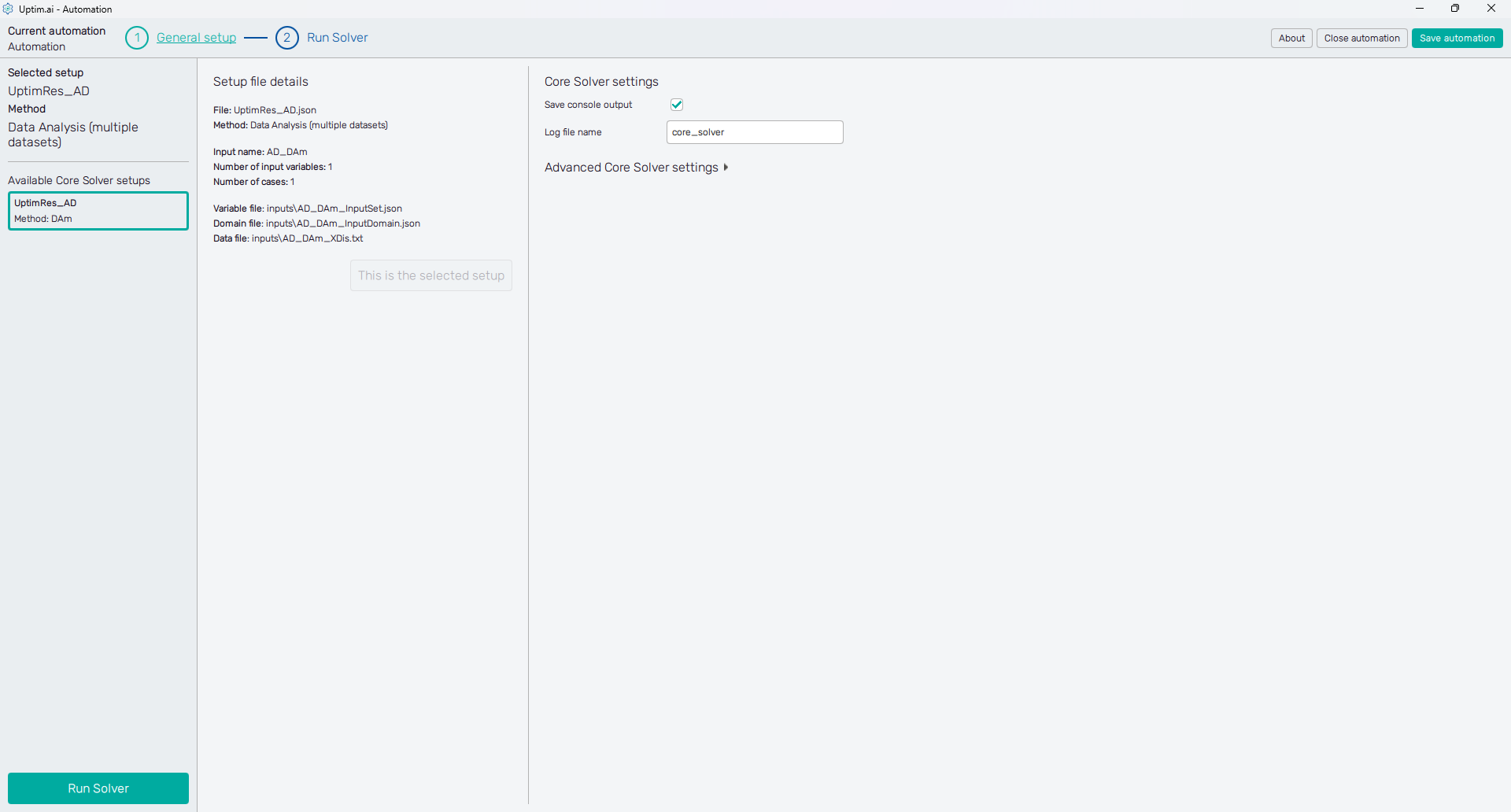
4.2: Select the Solver setup
The first important thing to do is to select the setup you've created in Part 3 of the tutorial. Our setup file UptimRes should be in the list of Available Core Solver setups shown on the left panel of the screen. The method 'DAm' (as Data Analysis - multiple datasets) was identified automatically to make the navigation through list items easier. Once the setup item is clicked, you can see the Setup file details. Then, confirm the selection with the Select this setup button.
4.3: Core Solver settings
The Core Solver settings is a simple task in this case. We recommend turning on the console output saving that stores the log of the Core Solver. There is no need to modify the advanced settings.
In this stage, the Run Solver button is active as well as the Run Solver item of the fishbone navigation bar at the top of the screen. Both of them lead to the next step.
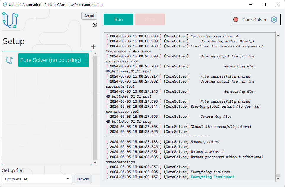
4.4: Run the Solver
As you can see at the top of the screen right under the fishbone navigation bar there is the Run Solver button with the status bar right next to it, saying Ready at the moment. Clicking the button runs the Core Solver that builds the mathematical model. The program will show the process log on the screen. Once the solver is running, the main button turns red, labelled Stop Solver until the mode is ready. This will be indicated by the 'Everything finalized' message at the end of the log.
Part 5: Result Postprocess
5.1: Open the Postprocessor
To see the results, we will open the Postprocessor from the Uptimai main interface.
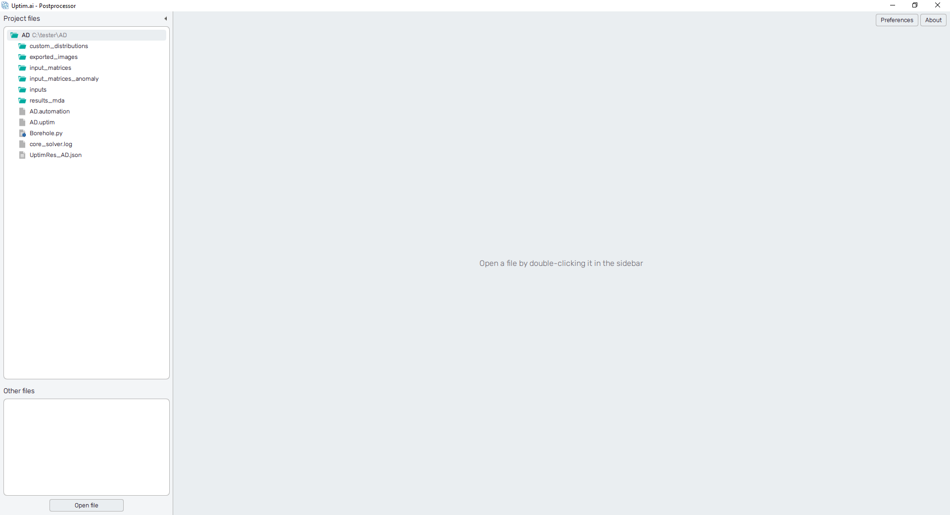
Now we will open the AD_O1_C1.upsg global result file. It is stored in the result_mda folder of the project
inside the sub-folder
called AD - the same as the prefix we choose for result files in the Core Solver Setup.
5.2: Pearson correlation
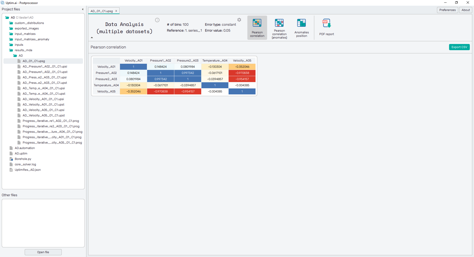
The default screen of the global result file of multiple datasets shows the table with Pearson correlations of all output combinations.
Clicking labels of the table directly opens the corresponding *.upst result file and accesses all
the corresponding post-processing features as described
here. Double-click inside the table opens a new
tab with the comparison of selected outputs.
5.3: Pearson correlation (anomalies)
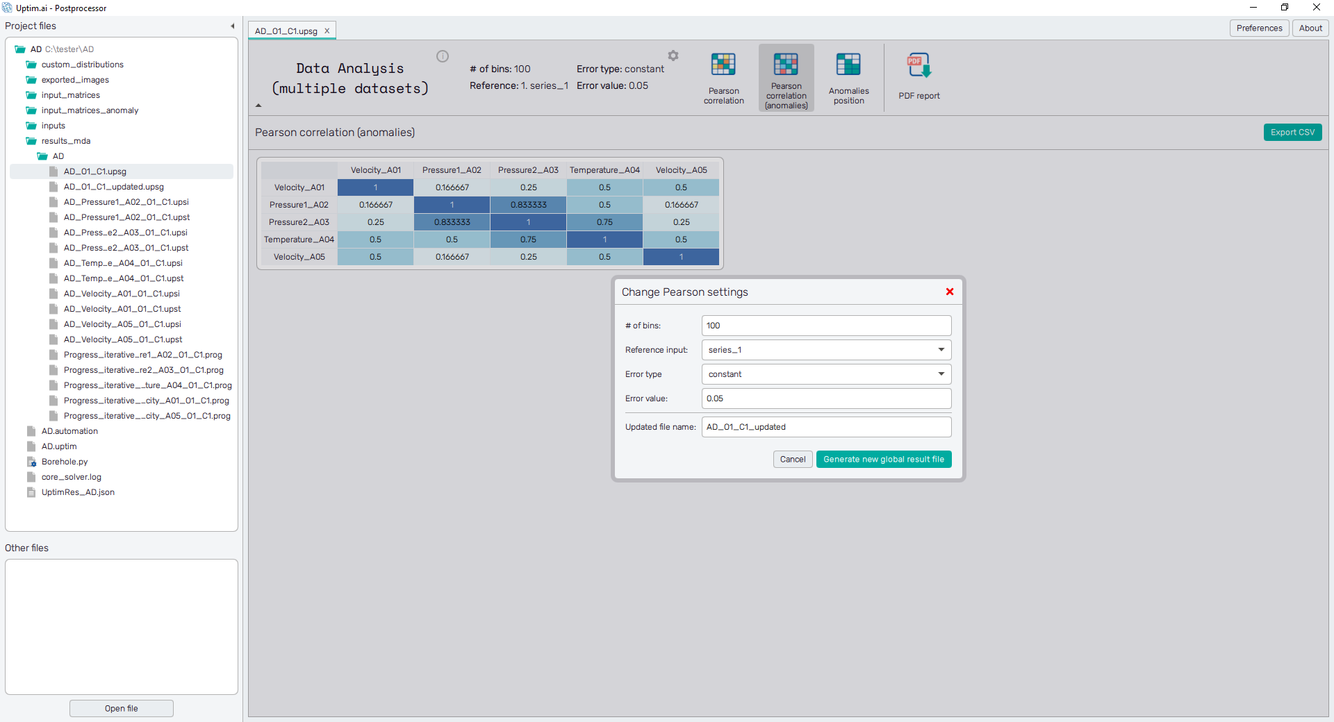
The next screen under the Pearson correlation (anomalies) icon reveals how is the distribution of anomalies correlated among the outputs. The table itself is organized in the same manner as on the previous screen, allowing direct access to the result file of each output or the comparison of the selected combination of outputs.
Values in the table represent the likelihood of an anomaly appearing at the same position for two different outputs. Open the Change Pearson settings dialogue with the ⚙ icon on the top of the window. You can try to change the values several times to see how these affect the number of identified anomalies.
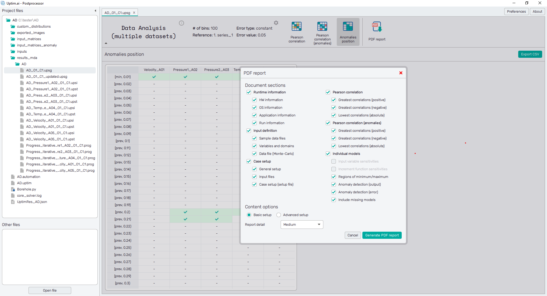
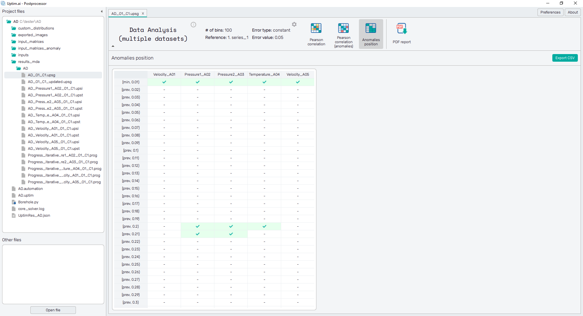
5.4: Anomalies position
Now, let's find out more about the anomalies, switching to the Anomalies position feature. Here you can see the table with locations of identified anomalies along the selected Reference variable. Anomalies marked in multiple columns on the same (or adjacent) row indicate the error is correlated for these outputs. The total number of listed anomalies is, of course, depending on the setup of the anomaly threshold. Scroll down with the mouse wheel to see the whole table.
5.5: Generate the PDF report
As the very last step, generate the report with the summary of all findings. Clicking the PDF report icon at the top bar of the window will directly show the dialogue with the report setup. Pay attention to all categories. Also, change the general Content options at the bottom of the page. Set the Report detail to Medium. If you are curious about the details of this setting, switch from the Basic setup to the Advanced setup.
The document will be created with the Generate PDF report button clicking.