Direct Optimization
This is a basic tutorial of Uptimai software, prepared to give a first introduction to the suite
and how to run its different features. To complete this tutorial, there will be needed the
Uptimai software and a *.zip file with some complementary files required for the example
problem to be solved. The Piston.zip file can be found inside the Uptimai Member Area ->
Downloads -> Tutorial cases.
The Piston.zip file contains the whole project folder, so the user can start at any step of the given
tutorial. Nevertheless, if the user wants to fulfil the tutorial from the beginning, only the
Python script Piston.py will be necessary, as all the other files will be generated
during the process.
This tutorial will show you:
- How to start the project
- How to run each program of the package
- What are the main features of each program, and how to use them
- What are the results you can expect
- How to export and store output data
Part 1: Launcher
1.1: Start the program
Open the Uptimai software. You can use the Start menu or desktop shortcut if this option was selected during the installation process, or find the executable inside the installation folder.
1.2: Begin the project
Create a New Project. You will have to choose an empty folder where all the project files will be located. The name of the folder will become the name of the project. In this example, we will use the name Piston. You can create the folder directly from the interface.
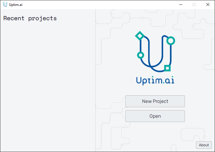
To switch between existing projects if needed, close the current one with the Close project button at the bottom left of the window and use the Open button of the Launcher (see Figure 1) to run another one.
Once you have created the project, a *.uptim file will appear inside your project folder.
That file is used as a flag so the folder is recognized as a Uptimai project, and contains
the information about already available sets of input files, setups, etc.
The basic rule for the
*.uptim file is that the file name has to be the same as the name of the project folder.
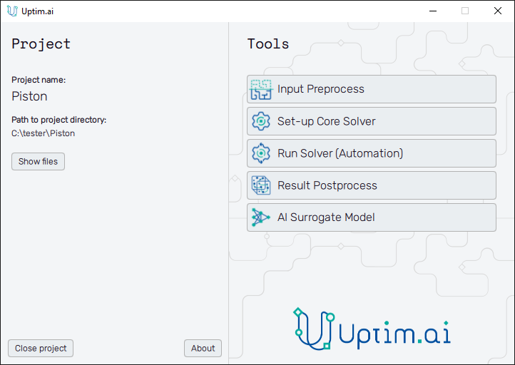
1.3: Proceed to Tools
Now, you have access to all the different features of the Uptimai suite. In this tutorial, we will use them one by one.
Part 2: Input Preprocess
2.1: Open the Input Preprocessor tool
The first step of all projects is always the Input Preprocessor, which can be opened directly from the main interface. The initial state can be seen in Figure 3.
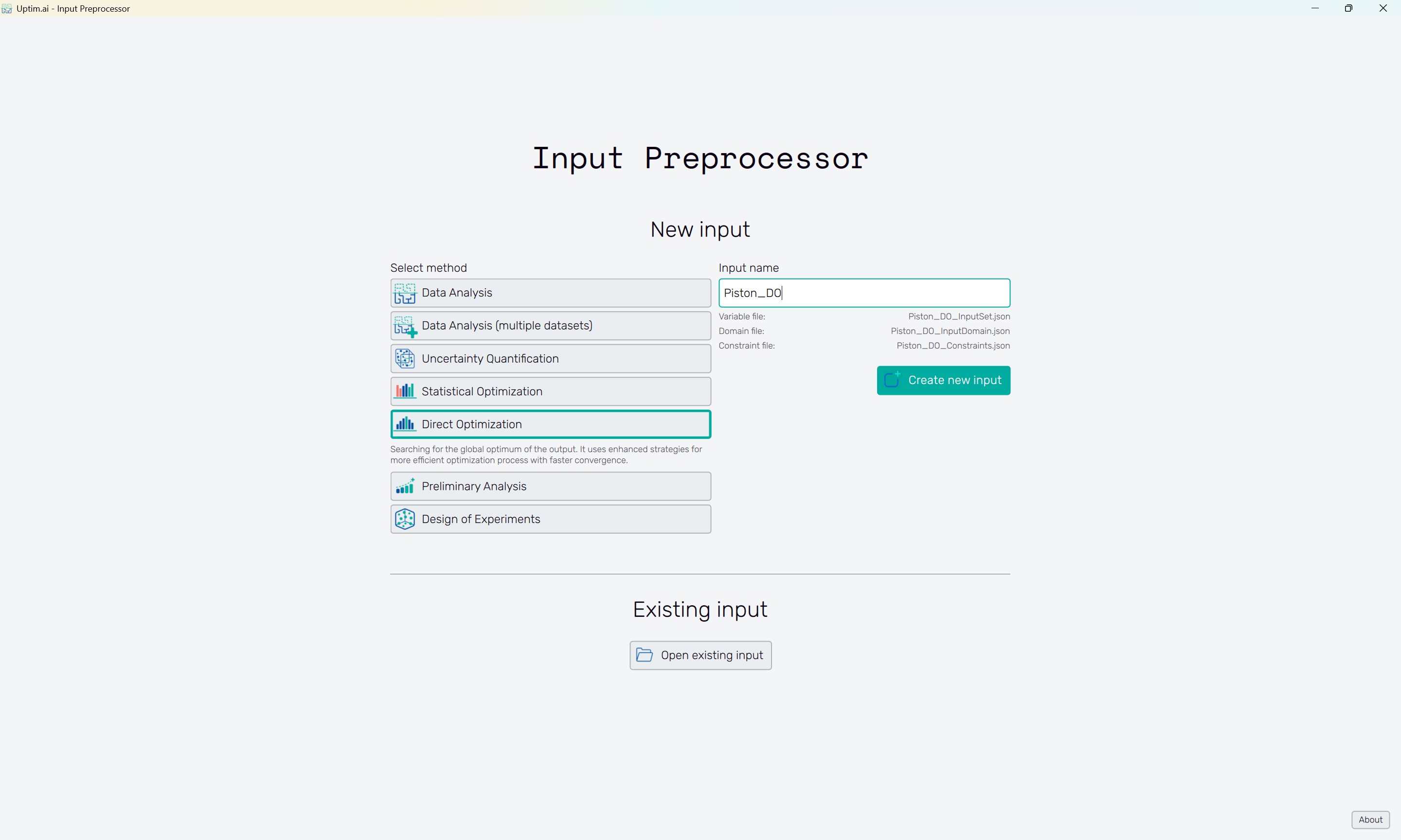
2.2: Inputs for the Direct Optimization method
In this tutorial, we will select the Direct Optimization method. It is possible to modify the Input name, but for simplicity, we will maintain the default name suggested by the software. Then, we can click the Create input button to start generating all the input files. You can see their names below the Input name entry.
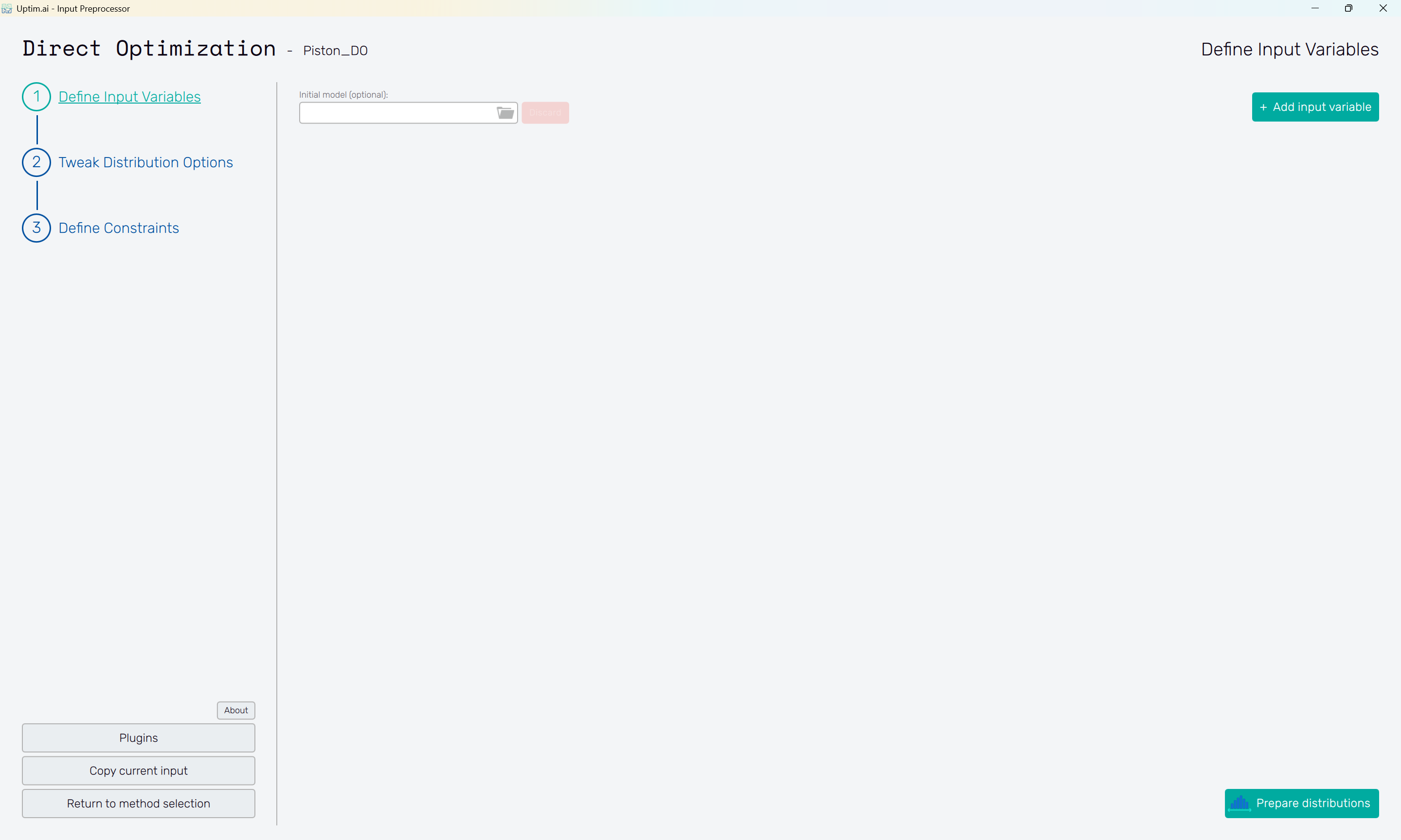
2.3: Add input variables
In this case, we have 7 input variables, so we will use the Add input variable button at the upper right to generate 7 variable spots.
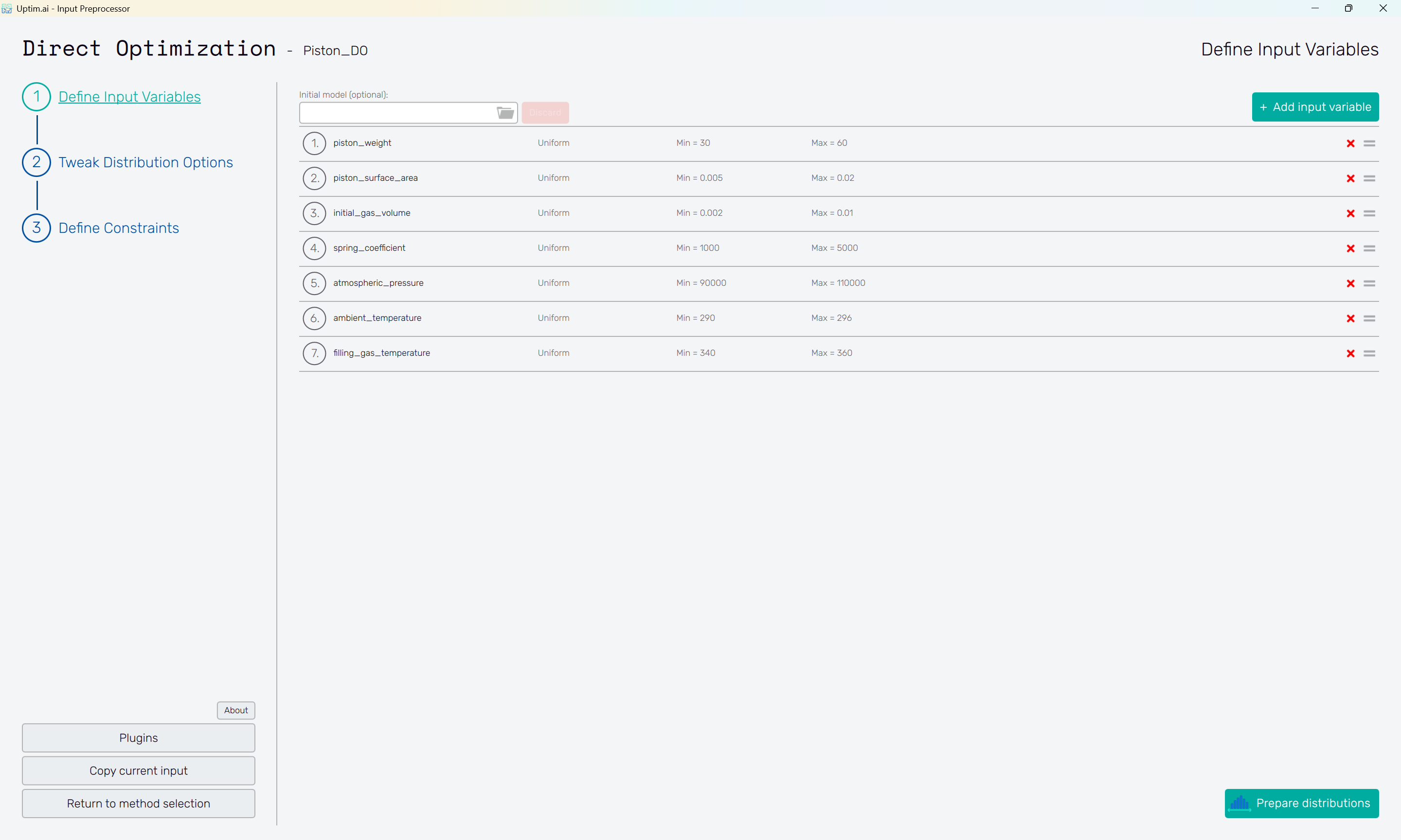
2.4: Define input variables
Insert the following distribution for each variable. Remember to press the Confirm button to save the changes after editing each variable. In the end, you should have the same settings as in Figure 5. Set the Activation type of all variables in the Advanced options menu to Active
The Prepare distributions button will generate all distributions according to the settings and then morph into the Tweak distribution options button.
Open to view Input Distributions
| Name | Type | Parameter 1 | Parameter 2 |
|---|---|---|---|
| piston_weight | Uniform | 30.0 | 60.0 |
| piston_surface_area | Uniform | 0.005 | 0.02 |
| initial_gas_volume | Uniform | 0.002 | 0.01 |
| spring_coefficient | Uniform | 1000.0 | 5000.0 |
| atmospheric_pressure | Uniform | 90000.0 | 110000.0 |
| ambient_temperature | Uniform | 290.0 | 296.0 |
| filling_gas_temperature | Uniform | 340.0 | 360.0 |
2.5: Prepare distributions
With all input variables defined completely, pre-generate random distributions of samples that will be later used for statistical analysis and visualizations. You can set the number of generated samples in the # of Monte-Carlo Samples entry at the top of the screen.
The Prepare distributions button will check the setup and then morph into the Tweak distribution options button.
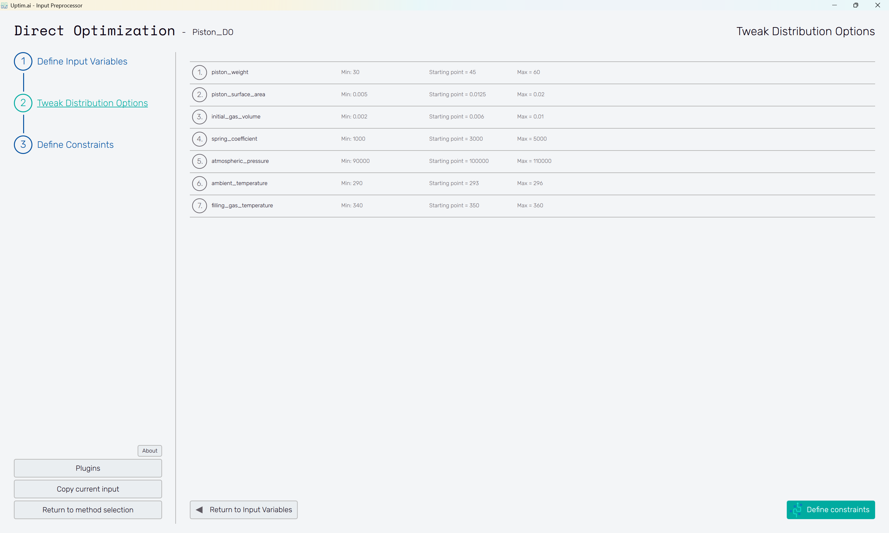
2.6: Tweak distribution Options
The Tweak distribution options button in the bottom right of the screen or the item of the fishbone navigation bar on the left brings the user to the Tweak Distribution Options screen. Boundaries of input distributions are adjusted here, as well as the position of the nominal sample.
By default, the nominal sample position is set to be the mean value of each input distribution. The nominal sample is, in general, used as a reference or starting point of the optimization. The setup is saved upon clicking the Generate data button, which also switches the screen to the next step of the workflow.
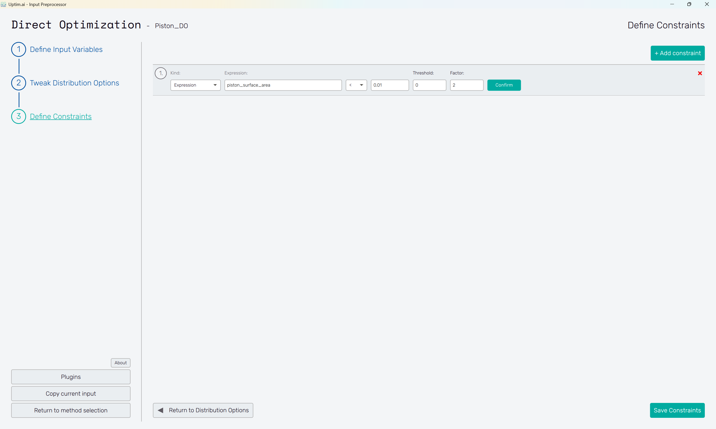
2.7: Define constraints
The next step is defining the constraints to be applied to input variables or outputs during the optimization process. Let's make a simple demonstration on variable piston_surface_area. The constraint will be defined as an Expression, stating there will be a penalty applied on the solution if the piston_surface_area is proposed larger than . Thus, the operator < is selected together with the value.
There is no Threshold allowed, and the Factor of is applied to the penalty score.
Part 3: Set up the Core Solver
3.1: Start the setup GUI
Once the inputs have been generated, it is time to prepare all the settings for the solver. We can do that using the Core Solver Setup, which, once opened from the Uptimai main interface, has the appearance as shown in Figure 10.
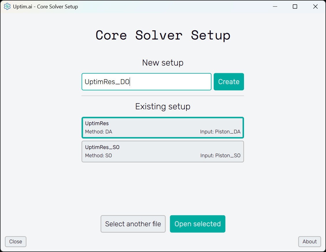
3.2: Create new setup
Once the program is opened, the first thing we need to do is to create a new setup file. We can change the name of the file to UptimRes_DO to directly address the used method, and then just click on the Create button.
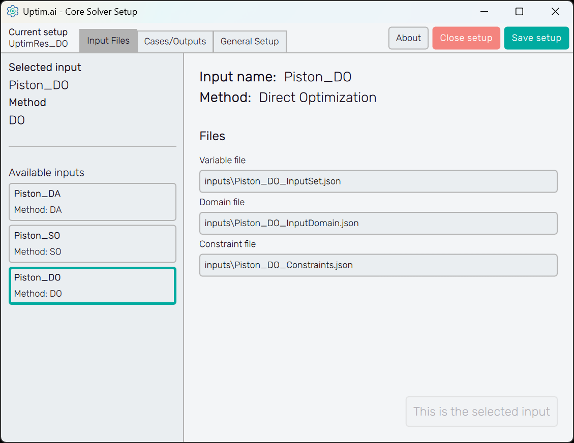
3.3: Select the set of inputs
Now, we will see that the Core Solver Setup has three main tabs. The first one is to select the input files that will be used in this run. In our case, we want to use the set of inputs prepared for the Direct Optimization method. Confirm the choice with the Select this input button.
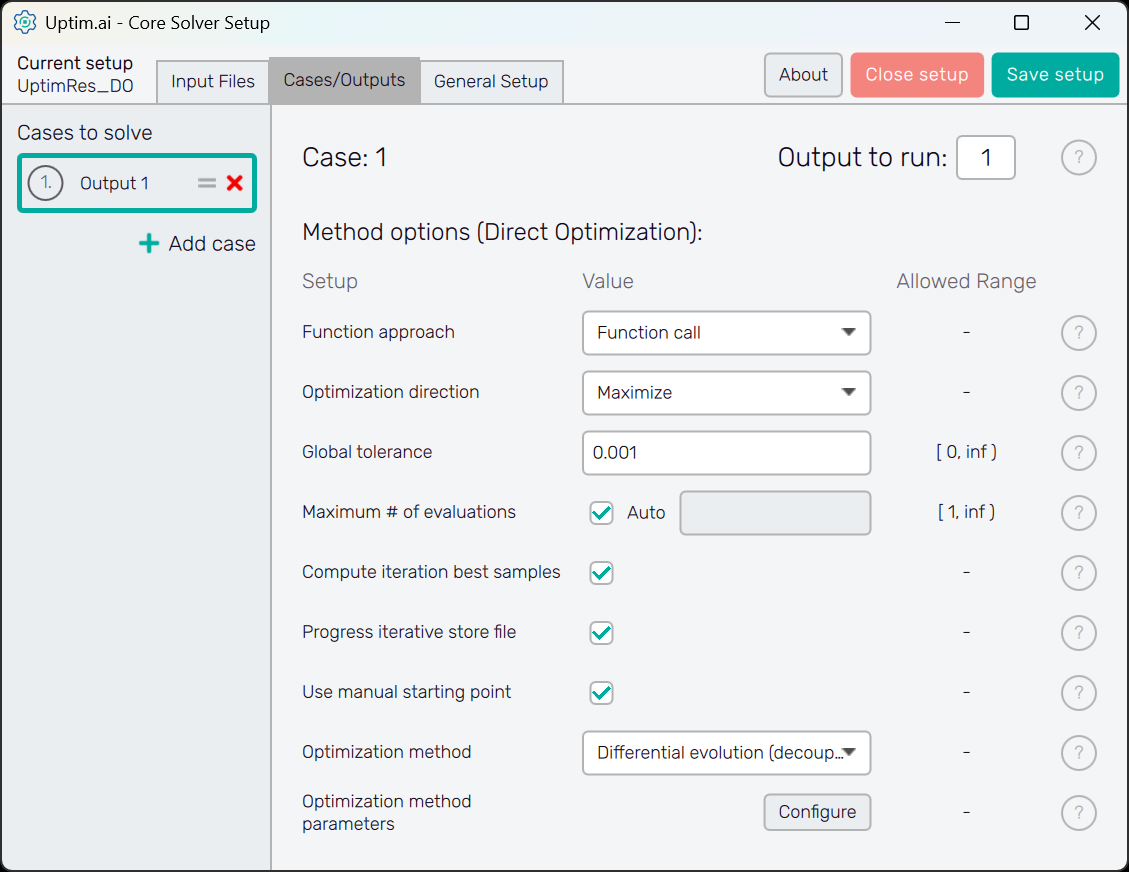
3.4: Set up the case
The second tab, which is Cases / Outputs, details all the settings that are used for tuning the core solver to the needs of each specific problem. Thus, there is a setup specific to the Direct Optimization method we are working with. Also, there is information about which outputs we would like to study. Only Output 1 is present at the start.
Here, we want to minimize the output that represents the piston cycle time. Set the Direction accordingly. Also, make sure the Function approach is set to Function call to allow the Uptimai Solver to be connected to our Python script. Let's also change the Optimization method to Differential evolution (decoupled). It is a modification of standard differential evolution optimization with increased efficiency. You can, of course, try out how all other methods work.
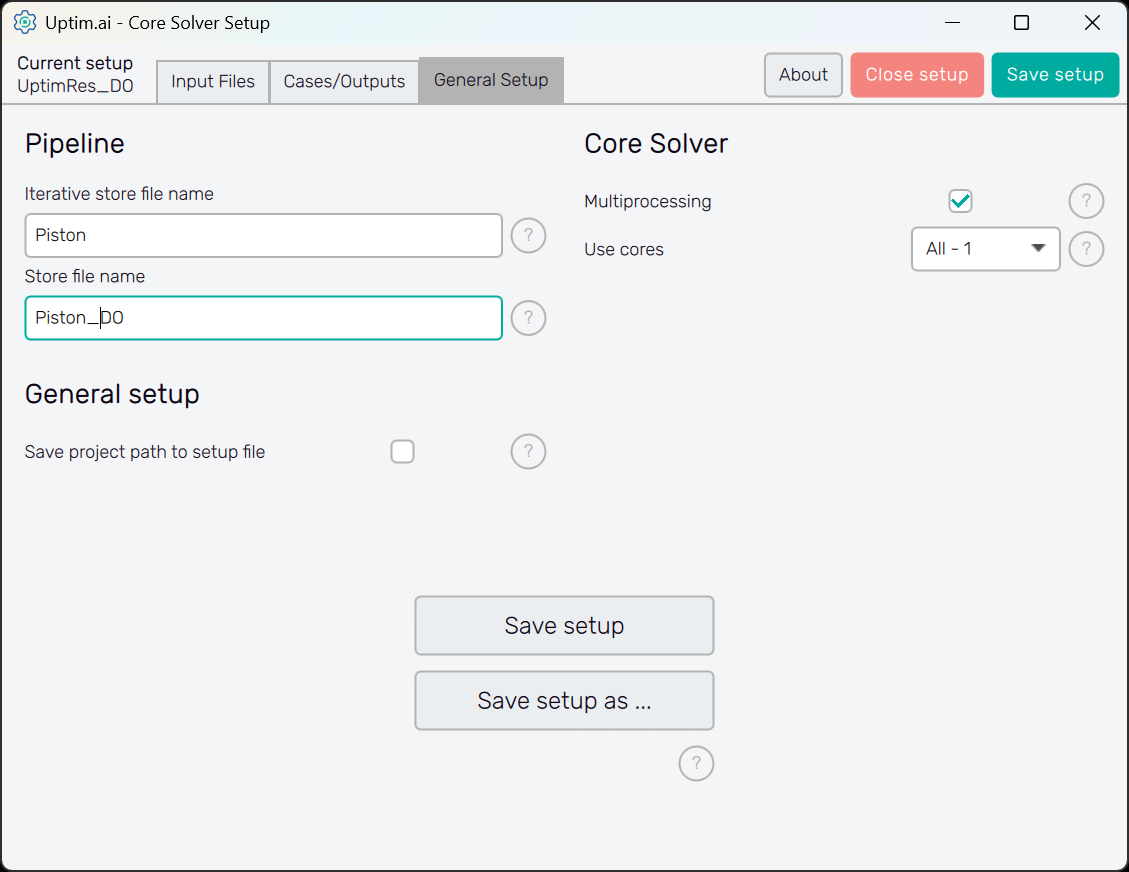
3.5: General setup
Finally, in the third tab, there is information regarding the naming of files and other solver aspects. In
this case, we can shorten the name of the output file prefix to Piston_DO and save the setup.
When we do that,
a UptimRes_DO.json file will be generated in the project folder containing all the information
that we saved. That file will be used by the solver itself.
Part 4: Run Solver (Automation)
4.1: Create new automation configuration
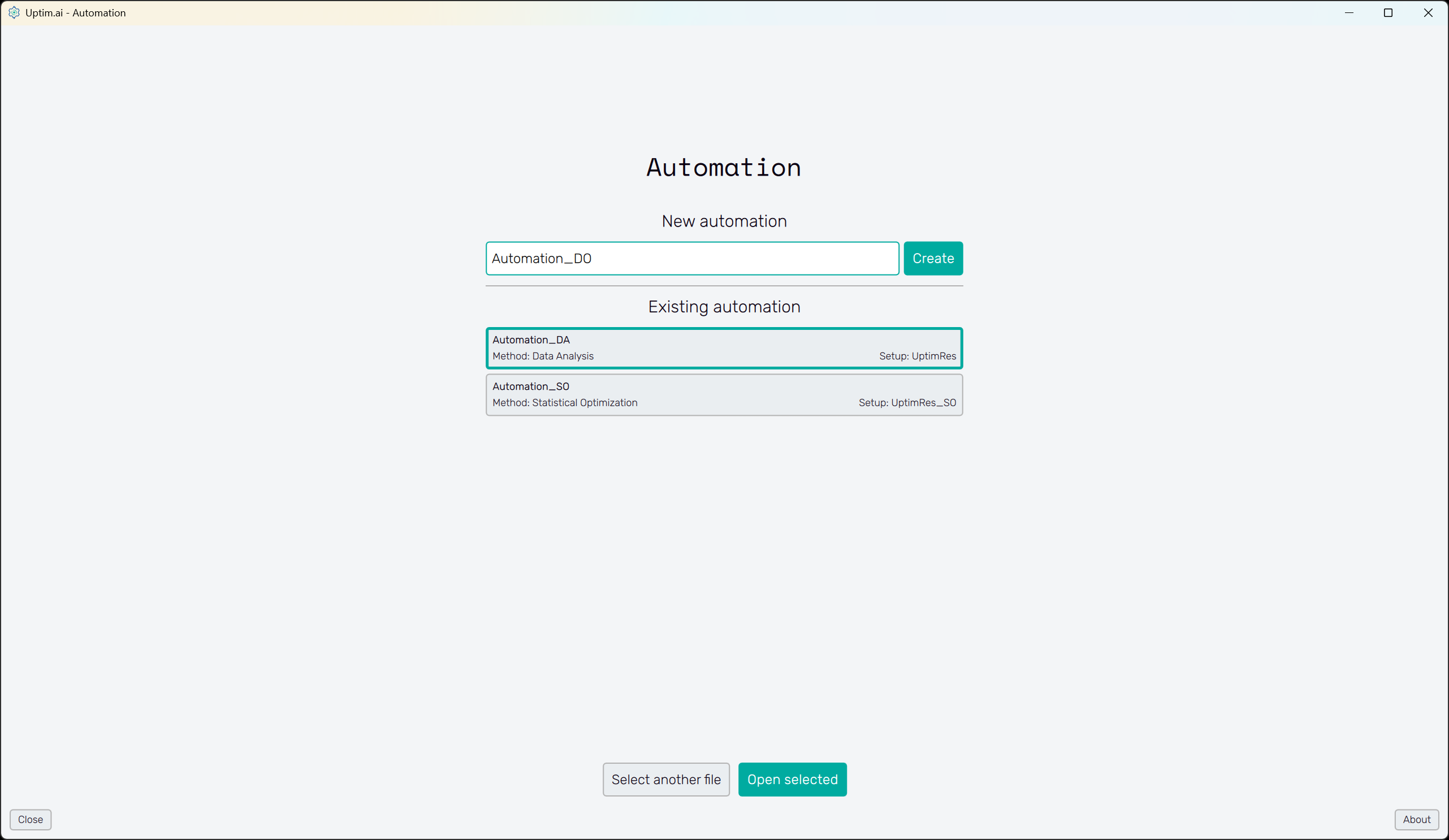
Now, it is time to open the Run Solver (Automation) from the Uptimai main interface. We will create a new automation file using the New automation section of the screen. Here, choosing any name and clicking the Create button stores the newly created file in the project folder. In case you want to load a previously created session, select one item from the list of the Existing automation section and confirm with the Open selected button. Eventually, you can search for any automation session under the Select another file button.
4.2: Add a connection
For Direct Optimization
cases using the Function call approach, there must be third-party software that converts a set of inputs
to a set of outputs, so we can adaptively create the model. In this tutorial, this role is taken by
a Python script called Piston.py that you can download from the
Member Area as a part of this tutorial project. Thus, the first step of this process would
be to download and paste the script into your project folder if you haven't already.
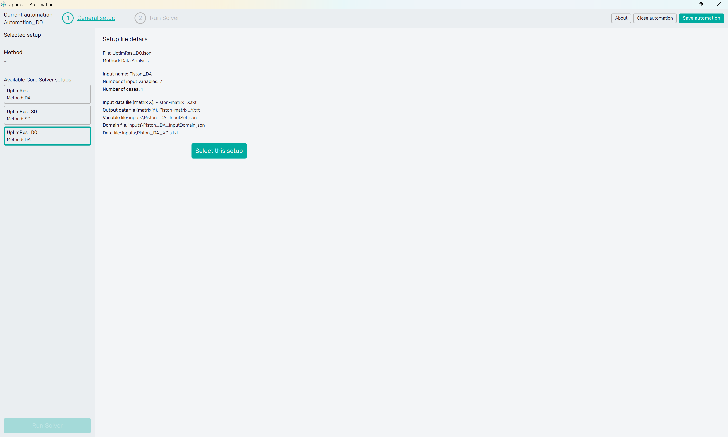
The next step is to select the setup you've created in Part 3 of the tutorial. Our setup file UptimRes_DO should be in the list of Available Core Solver setups shown on the left panel of the screen. The method 'DO' (Direct Optimization) was identified automatically to make the navigation through list items easier. Once the setup item is clicked, you can see the Setup file details. Then, confirm the selection with the Select this setup button.
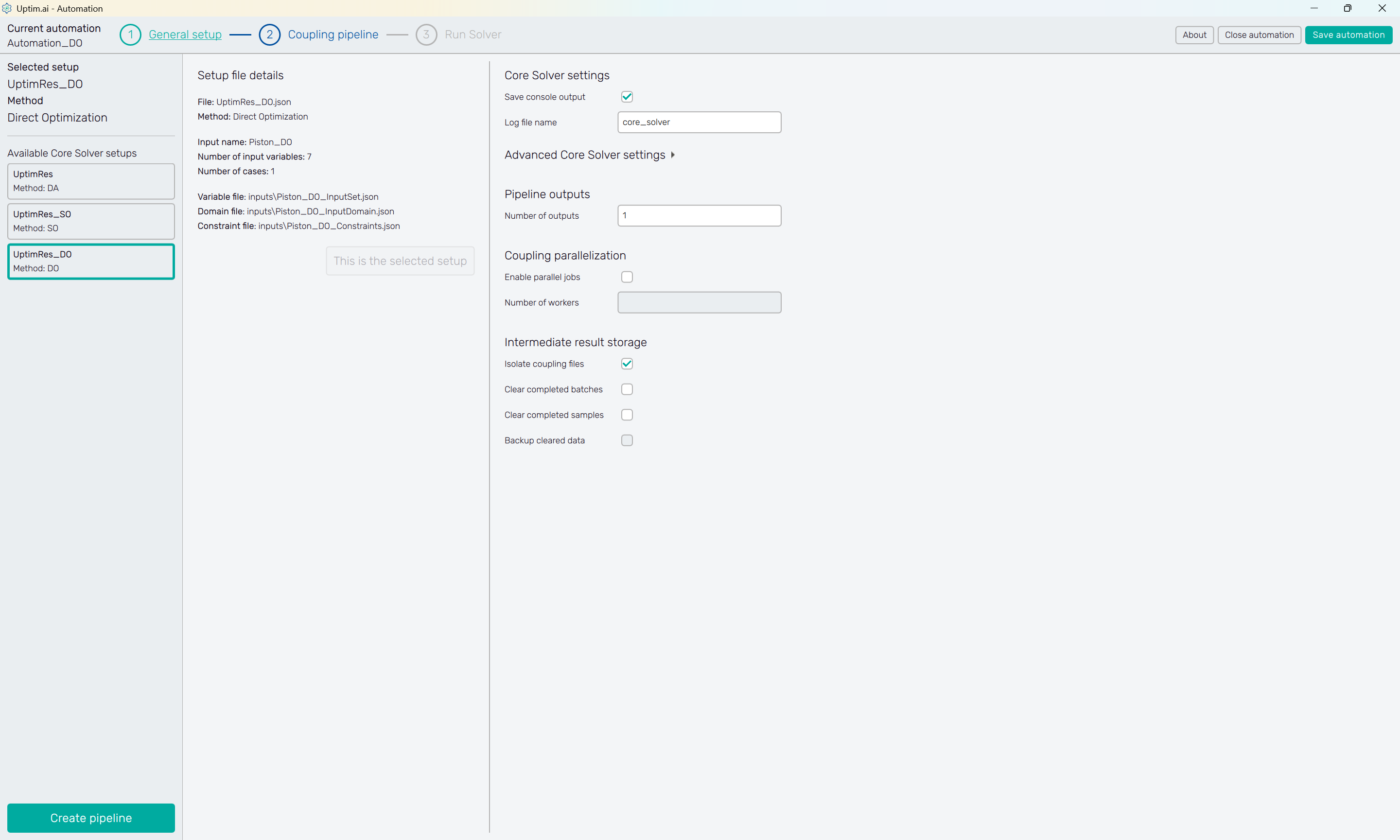
4.3: Core Solver settings
The Core Solver settings is a simple task in this case. We recommend turning on the console output saving, which stores the log of the Core Solver. There is no need to enter and set the Advanced Core Solver settings.
Since the Python script we are about to include in the pipeline has only one output, the Number of Outputs in the Pipeline outputs section can remain at its default state (). Try to switch the Enable parallel jobs in the Coupling parallelization on. Then, you can set the Number of workers for the parallel computation to speed up the process (we are using as an example).
Note that the Isolate coupling files switch was activated in the Intermediate result storage. As a result, a separate folder will be created in the project structure for each computed data sample. Keeping the data of pipelines running in parallel prevents them from overwriting each other's data, etc.
The Coupling pipeline button is active, as well as the Coupling pipeline item of the fishbone navigation bar at the top of the screen. Both of them lead to the next step.
4.4: Add Executable step to the pipeline
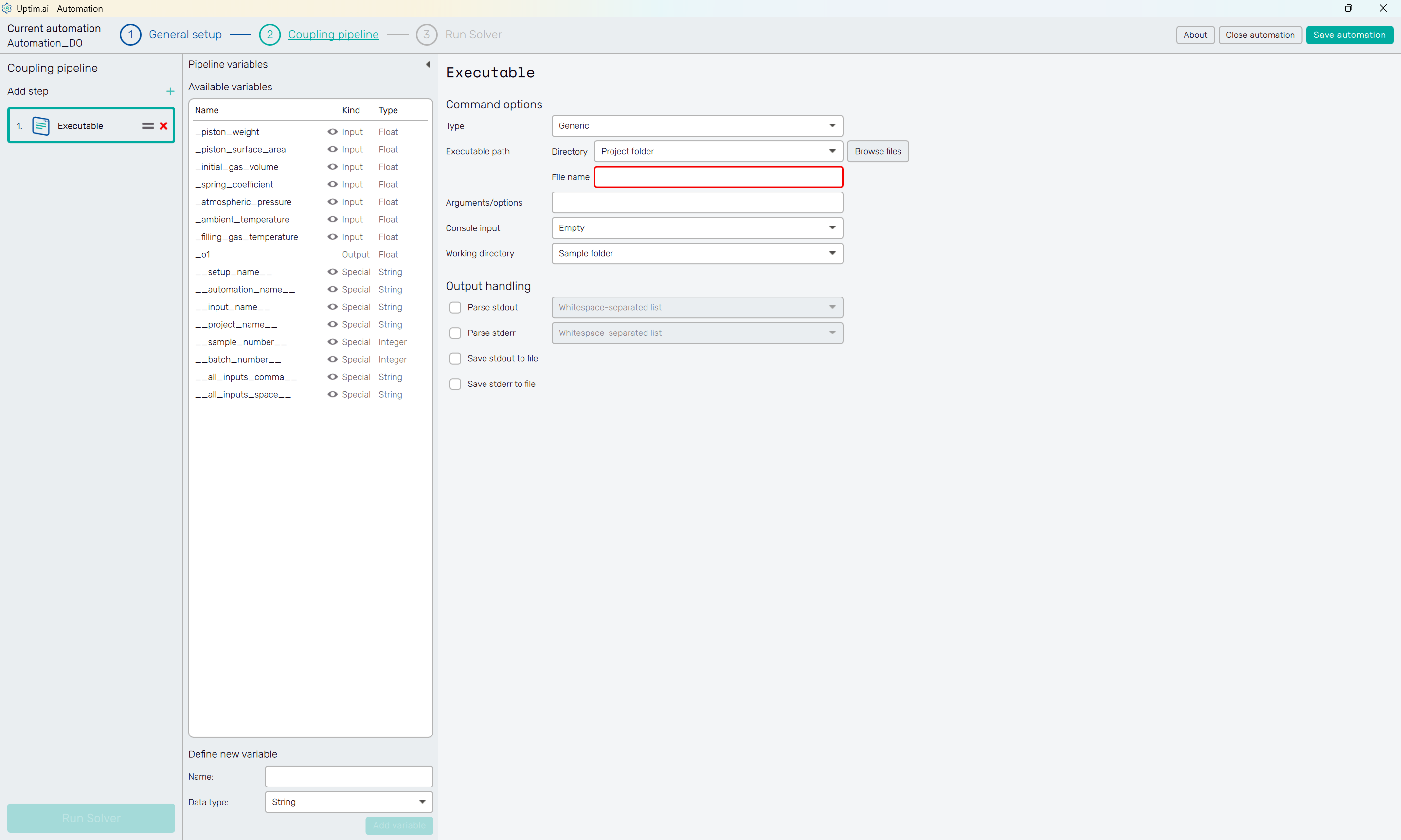
Figure 15 shows the initial state of the Coupling pipeline setup. At first sight, you can see the collapsible Pipeline variables panel holding the auto-generated list of Available variables, some of which will be used later in the process.
To the left, there is the Coupling pipeline itself. Click the + icon next to the Add step label and select the Executable item from the drop-down menu. This will add the Executable step to the pipeline.
4.5: Set the Python script connection
Under the Command options section, you need to change the Type to Python. Right after,
define the Executable path of our Piston.py file, which is expected to be in the Project folder.
The Project folder option should also be selected as the Working directory.
The crucial setting here is about passing values of input variables to the Python script, which expects
these arguments. The task here is to copy the names of all input variables enclosed in double curly brackets
to the Arguments/options entry in the correct order. Right-clicking on an item from the list of
Available variables shows the menu allowing the user to copy either the name of the variable or the formatted
name (with brackets). Use the advantage of the automatically created special variable __all_inputs_space__
that will load all inputs as space-separated values.
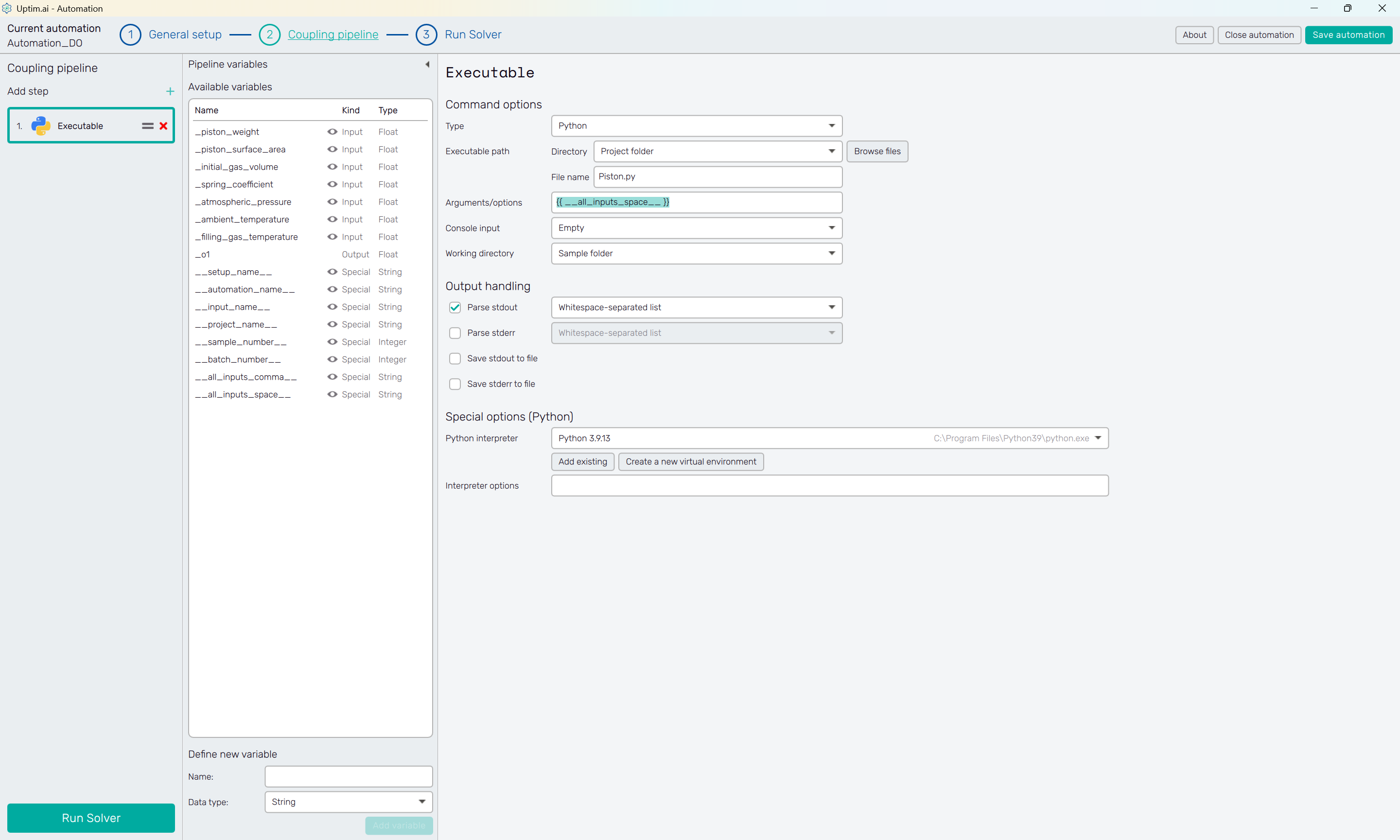
The last thing to set is selecting the Python interpreter in the Special options (Python) section. Be aware that the script is using the numpy library. Thus, this one should be available for the Python you are using.
Now, the Run Solver button is active as well as the Run Solver item of the fishbone navigation bar at the top of the screen. Both of them lead to the next step.
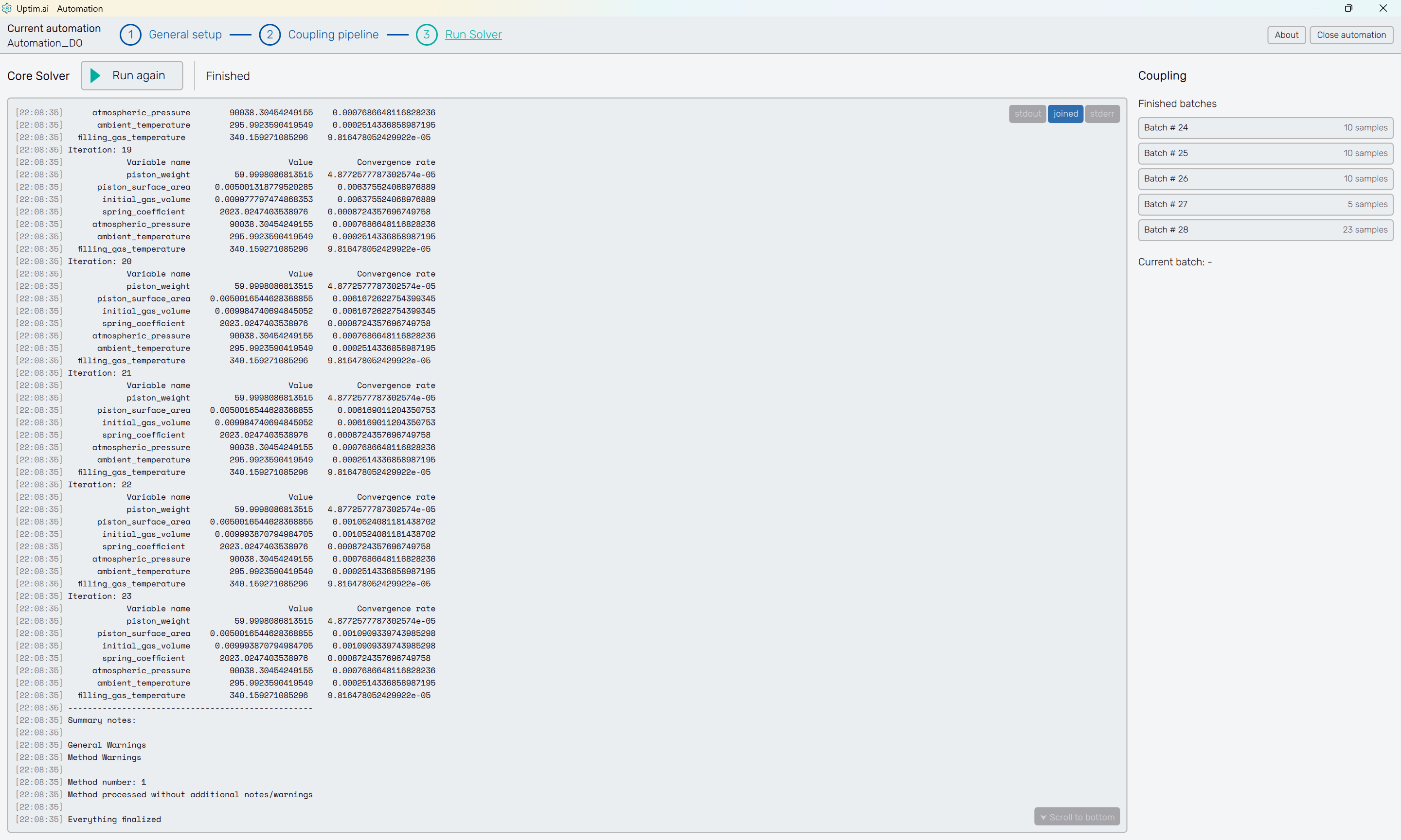
4.6: Run the Solver
Here comes the moment to click the Run Solver button at the top of the screen and wait until the solver finishes all tasks. The solver will automatically run the coupling pipeline for all needed samples and will build the model. An Everything Finalized message will appear at the end of the log when the solver is finished.
Part 5: Result Postprocess
5.1: Open the Postprocessor
To see the results, we will open the Postprocessor from the Uptimai main interface.
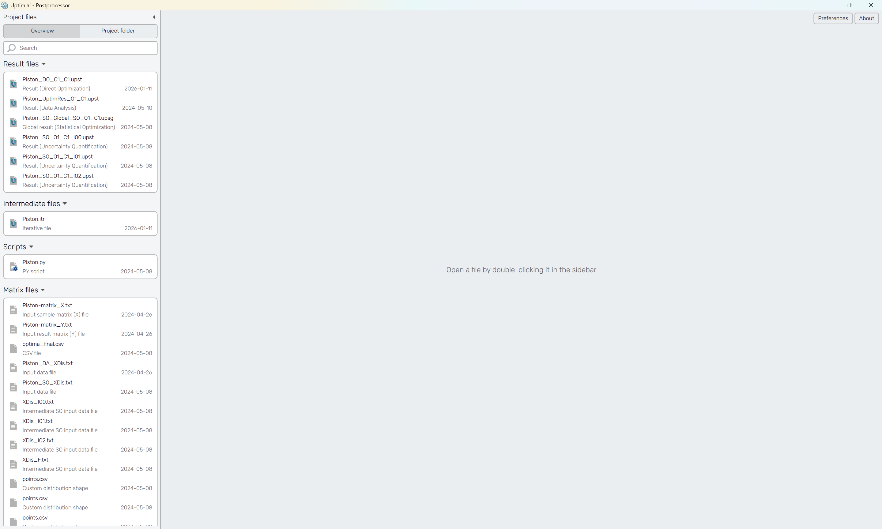
5.2: Open the Direct Optimization results
The *.upst file is available as the result of the
Direct Optimization method. Unless another name of the file
was chosen in the Core Solver Setup, the filename we are looking for is
Piston_DO_O1.upst.
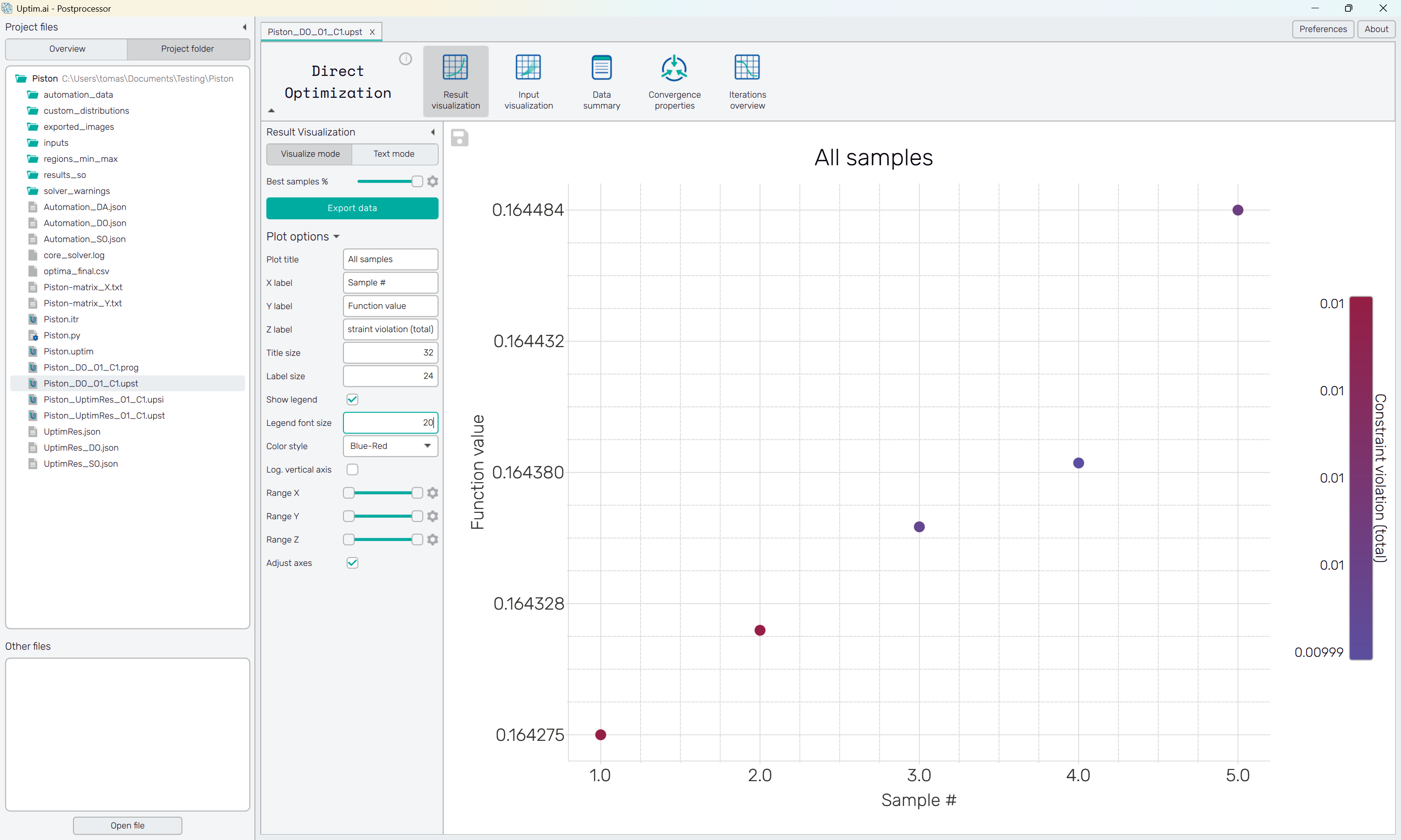
5.3: Result visualization
Check out the results of the last iteration of the optimization process. Samples of the last iteration are sorted here according to their function value. For each sample, details are available in a pop-up that appears when double-clicking on a selected sample. Besides the function value, it also indicates whether if some of the constraints were violated.
Switching to the Text mode shows the table with complete data, including input variable values of all samples in the plot.
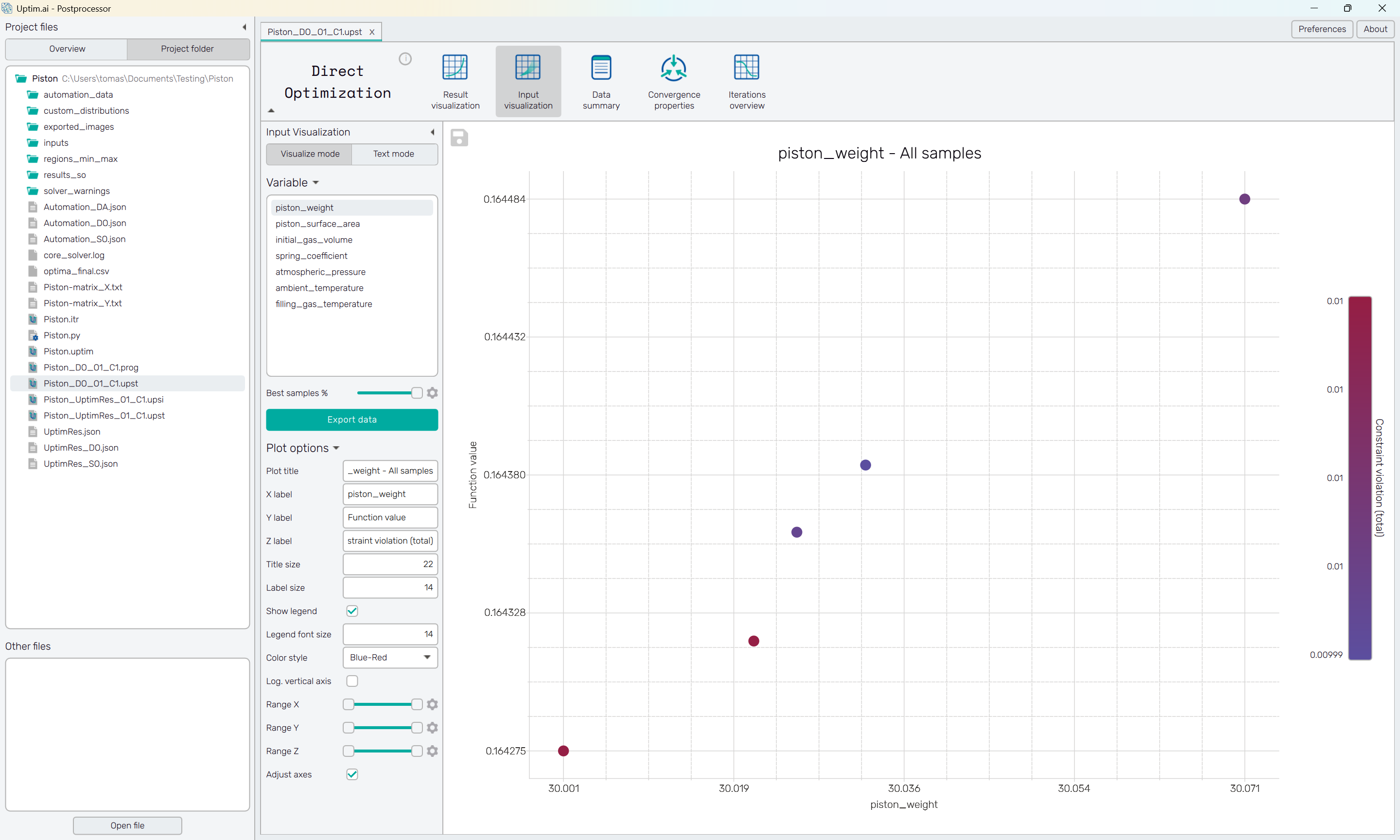
5.4: Input visualization
The second screen, Input visualization, shows samples of the last optimization iteration with respect to input variable values. Select the desired input variable from the list on the left to see the distribution of optimized samples along the range of the selected input.
Switching to the Text mode shows the table with complete data, including input variable values of all samples in the plot.
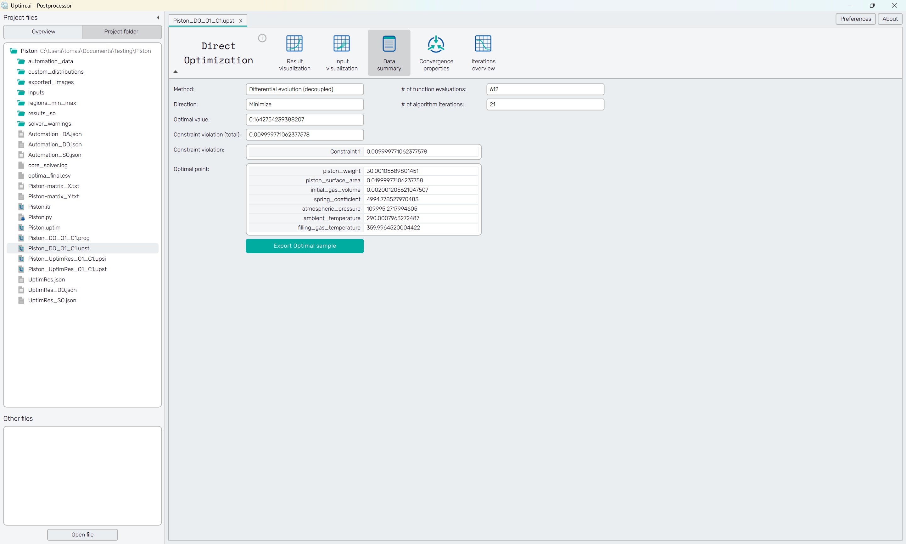
5.5: Data summary
To see the overall information about the optimization process, see the Data summary page. Along with the found global optimum, it gives the number of iterations and function evaluations required to obtain the result. Of course, there are coordinates of the optimal sample, locating it in the design space.
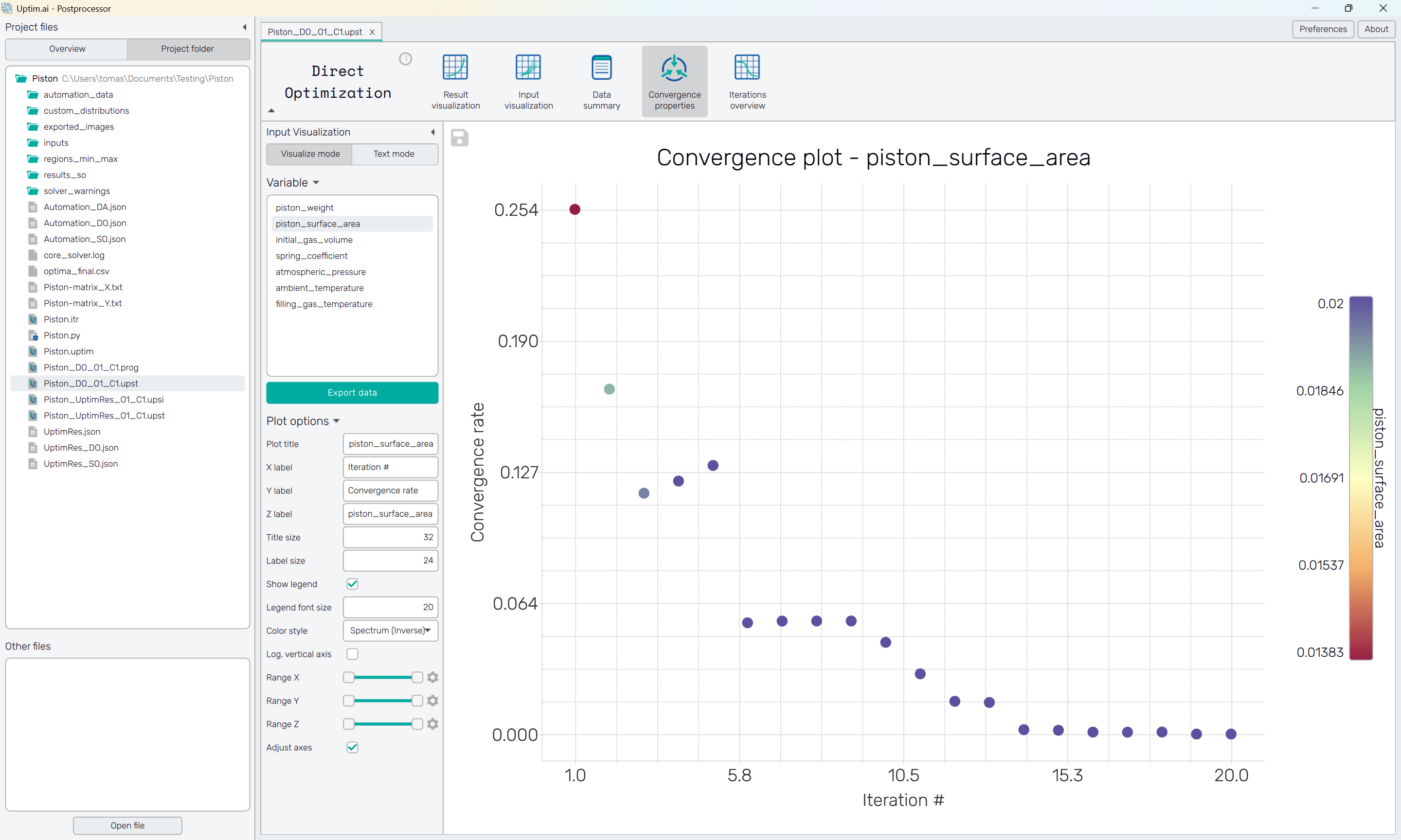
5.6: Convergence properties
An even more detailed breakdown of the optimization process is available in the Convergence properties plot. It shows the convergence rate from iteration to iteration for the input variable selected from the list on the right. See the input variable value related to the best sample of each iteration, which will give you a better idea of how the optimizer proceeded.
Also, this feature has the Text mode showing the complete table of values for all iterations, too.
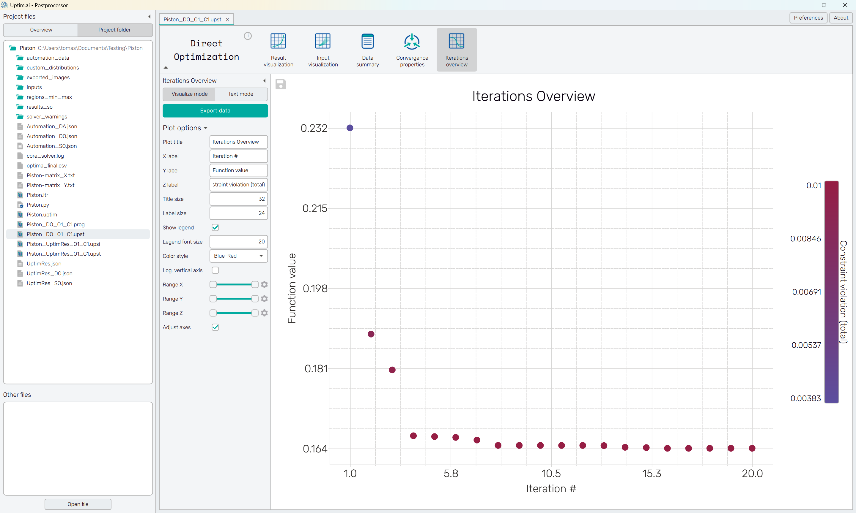
5.7: Iterations overview
Finally, the complete overview of all optimization iterations is available under the last icon of the top bar. In its Visualize mode, it shows how the function value changed along the process. The color of the samples indicates the constraint violation eventually present in a sample.
The Text mode shows the complete table of values for all iterations.