Direct Optimization

The Uptimai Direct Optimization focuses on finding the optimum of a given problem. Unlike the Statistical Optimization approach, it does not build any intermediate surrogate models — instead, it directly explores the design space using robust, well-established optimization algorithms such as Differential Evolution (DE), CMA-ES, Nelder-Mead, and GSS.

To further increase efficiency, the method applies a function decoupling strategy, where the problem is intelligently separated into smaller, lower-dimensional subproblems that can be solved independently. This significantly reduces the number of required samples while maintaining high accuracy in the search for the optimum. Moreover, in high-dimensional spaces, it tends to reach higher-quality optima than simple optimizers.

Direct Optimization can operate in two modes: in can interface with external engineering software to compute outputs for requested parameter combinations, or it can leverage an existing surrogate model created using the Uptimai Data Analysis or Uncertainty Quantification method to evaluate samples directly.

How to use the interface

The general appearance of the program window, especially its left section, is described in detail in the Input preparation link. Here the main focus is on the other part which is to a certain point individual for each of the supported methods. The initial of the GUI window when preparing inputs for the Direct Optimization is shown in Figure 1, as the user starts from scratch and needs to Define Input Variables.

Define Input Variables

Figure 1: Direct Optimization - Initial state of the Input Preprocessor window

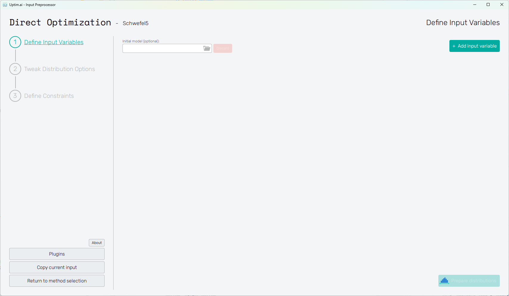
In the beginning, only one control is available for the user:

• Add input variable : Creating a new variable (parameter) of the input domain. Each added variable appears at the bottom of the list of already existing variables.

Figure 2: Direct Optimization - Definition of an input variable

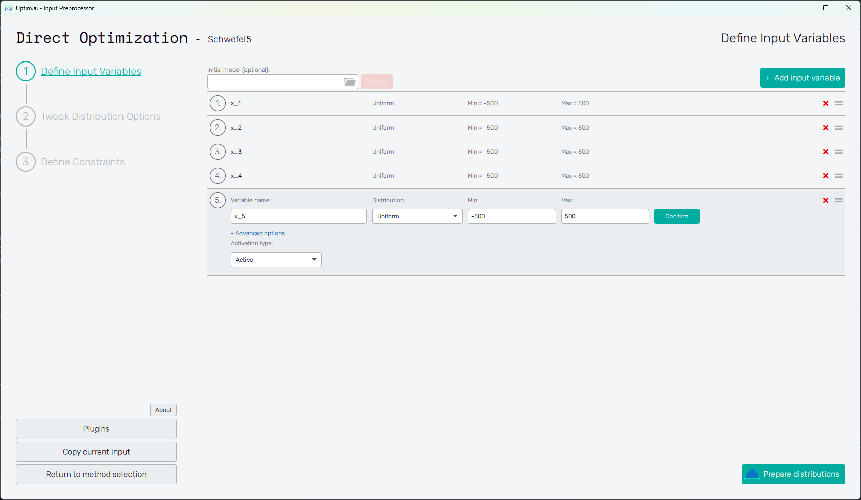
Adding an input variable enhances the input domain space with one dimension. There has to be at least one variable to optimize. Figure 2 describes the situation with multiple input variables already created (see this link for more info about the Schwefel Function used here as an example). One of the displayed variables is about to be edited. The input variable can be set using the following controls:

• Variable name : Label of the input parameter, which is being used throughout the whole process up to the postprocessing. The variable name cannot contain empty spaces, these are automatically replaced with underscores.
  • Distribution : Selection box where the user sets the shape of the probabilistic function for the input variable. According to the distribution type selected, additional entries with shape parameters appear. A detailed description of featured probability distribution types can be found in the section Input distribution types.
  • Confirm : Any changes need to be confirmed with this button to take effect.
  • "X" : Each input variable can be deleted when clicking this icon.
  • "=" : Allows input variable dragging to change the ordering of inputs in the projects.
  • "+ Advanced Options:
  • Activation Type" : Allows change between Active (by default) and Inactive. Active means that the intrinsic uncertainty of the variable will be propagated and Inactive means that only the nominal value will be used (variable won’t be studied).

Adding one or more input variables activates the Prepare distributions button. This one invokes the preparation of randomly distributed samples according to the settings. In case there are invalid entries in the input variable definition, the user is informed and not allowed to continue to the next step until everything is by the book. Then, the button itself turns into Tweak distribution options, sending the user to this next step. Also, the Tweak Distribution Options item is activated in the fishbone navigation bar on the left.

Initial model

In the top area, the user can choose the "Initial model" - that is a ".upsi" file produced by the Core Solver by running the Data Analysis or the Uncertainty Quantification method. In case the initial model is selected, all variables are loaded from the model and cannot be edited anymore (the only exception being the Activation type).

Setting the initial model is required, if the user intends to use the "Data model" function approach later in the Core Solver Setup. If that is the case, instead of calling an actual function using coupling, all samples will be evaluated using the selected model. For further details, check the Core Solver Setup documentation.

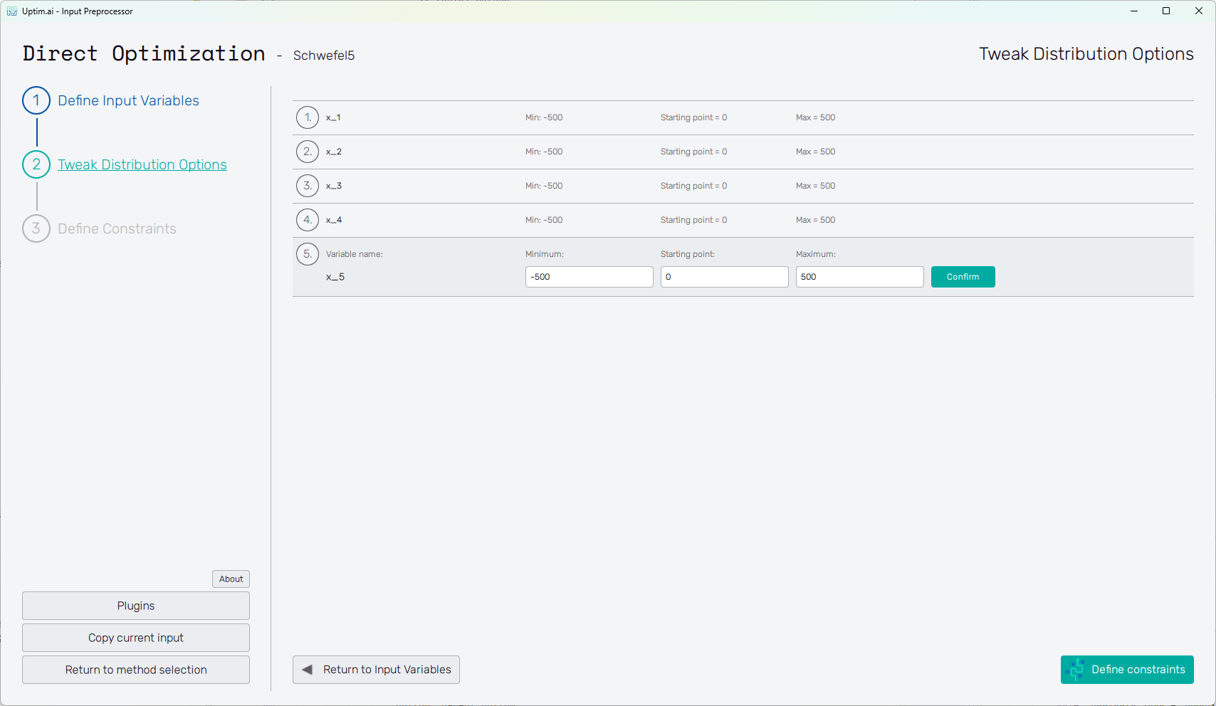
Tweak distribution options

At this point, the user adjusts the so-called starting point. The starting (or central) point is a sample acting as a baseline for the analysis. The results of all data samples are compared with the result value of the nominal sample. This process allows handling the effects of input parameters and their interactions separately as increments to the nominal value. It must be within the range of each input variable and may be equal to its boundaries. Although not strictly necessary, it is recommended to place the nominal sample into the statistical centre of the domain. Then, the process of the optimization is most efficient and precise. The central sample's default position is suggested as the mean of the probability distribution of each input variable. When changing its position, (shown in Figure 3) it is advised to not shift it by more than 10% of the range of each input. As in the case of input variable distribution definition, all changes must be saved using the Confirm button.

Figure 3: Direct Optimization - Tweaking input distributions

Special considerations

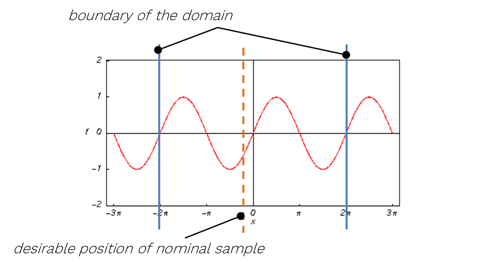
For the sampling of variables leading to periodic or symmetrical functions (typically, but not exclusively, angles of any kind), extra caution is required. It is highly recommended not to set their nominal value exactly to the centre of symmetry of the corresponding input distribution! A typical example can be the angular position of a crankshaft, wave phase, etc.

At the bottom right there is a Define Constraints button. If everything on the page is set correctly, it will send the user to this next step. Also, the Define Constraints item is activated in the fishbone navigation bar on the left.

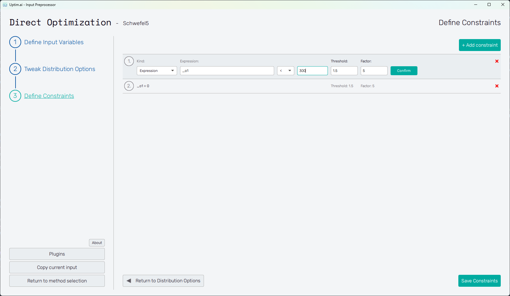
Define Constraints

This page allows the user to specify mathematical constraints that limit the design space explored during the optimization process. Constraints can be defined as either equalities (e.g. x_1 + x_2 = 0) or inequalities (x_1 < x_2). These expressions restrict the optimization to feasible regions of the problem domain.

Figure 4: Direct Optimization - Defining constraints

The constraint expressions can be built using:

• Input variables
• Function outputs
• A set of mathematical functions
  • sin, cos, tan, arcsin, arccos, arctan, arctan2, sinh, cosh, tanh, sinc, arcsinh, arccosh, arctanh, floor, ceil, trunc, exp, exp2, log, log2, log10, sqrt, cbrt, abs, sign
• Alternatively, the constraint can be defined using a Python script

Each constraint includes two additional parameters:

• Factor - defines how strongly a constraint violation is penalized. A higher factor increases the penalty applied to samples that do not meet the condition.
• Threshold - defines a tolerance margin ("grace area"). Small deviations within this range are ignored and do not contribute to the penalty.

If a constraint is not satisfied, a penalty is applied to the objective function according to the following equations:

$$\begin{aligned} p_{\text{eq}} &= \lvert c(x, f(x)) - \text{target} \rvert \\ p_{\text{ineq}} &= c(x, f(x)) - \text{target} \\ p_{\text{thres}} &= \begin{cases} 0, & \text{if } p < \text{threshold} \\ p, & \text{otherwise} \end{cases} \\ penalty &= \sum (\text{factor} \times p_{\text{thres}}^2) \\ f_{\text{penalized}} &= \begin{cases} f(x) + penalty, & \text{if } \text{direction} = \text{minimize} \\[4pt] -\bigl(-f(x) + penalty\bigr), & \text{if } \text{direction} = \text{maximize} \end{cases} \end{aligned}$$

Defining the constraint using expression

When the user selects the "Expression" constraint kind in the first field, they are presented with the following additional fields:

• Expression - used to define the expression using the variable names, function outputs (_ox, where x = 1, 2, ...) and mathematical functions mentioned above.
• </= - select < for inequality or = for equality.
• r-value - a real number. The constraint is then defined as <expression> [<|\=] <r-value>.
• Threshold - tolerance margin, a real number.
• Factor - penalty multiplier, a positive real number (if set to zero, the constraint is effectively disabled).

Figure 5: Direct Optimization - Defining the constraint using a mathematical expression

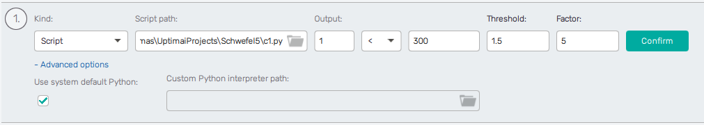
Defining the constraint using script

When the user selects the "Script" constraint kind in the first field, they are presented with the following additional fields:

• Script path - an absolute to the Python script
• Output - in case the script outputs multiple values, this selects which one will be considered.
• </= - select < for inequality or = for equality.
• r-value - a real number. The constraint is then defined as <script_outputs>[output] [<|\=] <r-value>.
• Threshold - tolerance margin, a real number.
• Factor - penalty multiplier, a positive real number (if set to zero, the constraint is effectively disabled).
• Advanced options - by default, the "system default" Python interpreter is used to evaluate the constraint script. The user can select a different interpreter.

Figure 6: Direct Optimization - Defining the constraint using a Python script

The example structure of the script is the following:

import numpy as np
import numpy.typing as npt

def eval_constraints(samples: npt.NDArray[float], func_values: npt.NDArray[float]) -> npt.NDArray[float]:
	cons_out_1 = np.log(samples[:, 1:2] - samples[:, 3:4])
	cons_out_2 = (func_values[:, 0:1] - np.mean(func_values[:, 0:1])) ** 2
	return np.concatenate((cons_out_1, cons_out_2), axis=1)

• The script must contain a function named eval_constraints, which:
  • Accepts two numpy arrays as arguments: the samples (x) and their function values (f(x)).
    • The shapes are (n, n_var) and (n, n_out), where n is the number of samples, n_var is the number of variables and n_out is the number of function outputs
  • Returns a single numpy array (the constraint values of the input samples)
    • The shape is (n, n_cons_out), where n is the number of samples and n_cons_out is the number of constraint outputs
• The script can also contain different helper functions and classes that are used in the process
• In most cases, the number of constraint outputs is expected to be 1. However, in case multiple constraints have e.g. common intermediate values that are used during the computation, it may be useful to define them as multiple outputs in one constraint script, as the results of constraint script evaluations are cached.

note

The constraints are evaluated for each batch of samples during the optimization process. This will happen once per iteration and both the batch size and number of iterations will change depending on the global optimization process configuration. The number of samples in a batch can also differ across iterations.